| Oracle® Database Data Warehousing Guide 10g Release 1 (10.1) Part Number B10736-01 |
|


|
View PDF |
| Oracle® Database Data Warehousing Guide 10g Release 1 (10.1) Part Number B10736-01 |
|
|
View PDF |
This chapter discusses query rewrite in Oracle, and contains:
One of the major benefits of creating and maintaining materialized views is the ability to take advantage of query rewrite, which transforms a SQL statement expressed in terms of tables or views into a statement accessing one or more materialized views that are defined on the detail tables. The transformation is transparent to the end user or application, requiring no intervention and no reference to the materialized view in the SQL statement. Because query rewrite is transparent, materialized views can be added or dropped just like indexes without invalidating the SQL in the application code.
A query undergoes several checks to determine whether it is a candidate for query rewrite. If the query fails any of the checks, then the query is applied to the detail tables rather than the materialized view. This can be costly in terms of response time and processing power.
The optimizer uses two different methods to recognize when to rewrite a query in terms of a materialized view. The first method is based on matching the SQL text of the query with the SQL text of the materialized view definition. If the first method fails, the optimizer uses the more general method in which it compares joins, selections, data columns, grouping columns, and aggregate functions between the query and materialized views.
Query rewrite operates on queries and subqueries in the following types of SQL statements:
SELECT
CREATE TABLE … AS SELECT
INSERT INTO … SELECT
It also operates on subqueries in the set operators UNION, UNION ALL, INTERSECT, and MINUS, and subqueries in DML statements such as INSERT, DELETE, and UPDATE.
Several factors affect whether or not a given query is rewritten to use one or more materialized views:
Enabling or disabling query rewrite
By the CREATE or ALTER statement for individual materialized views
By the initialization parameter QUERY_REWRITE_ENABLED
By the REWRITE and NOREWRITE hints in SQL statements
Rewrite integrity levels
Dimensions and constraints
The DBMS_MVIEW.EXPLAIN_REWRITE procedure advises whether query rewrite is possible on a query and, if so, which materialized views will be used. It also explains why a query cannot be rewritten.
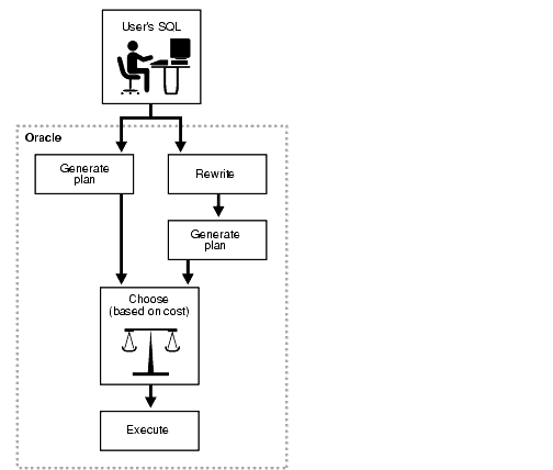
Query rewrite is available with cost-based optimization. Oracle Database optimizes the input query with and without rewrite and selects the least costly alternative. The optimizer rewrites a query by rewriting one or more query blocks, one at a time.
If query rewrite has a choice between several materialized views to rewrite a query block, it will select the ones which can result in reading in the least amount of data. After a materialized view has been selected for a rewrite, the optimizer then tests whether the rewritten query can be rewritten further with other materialized views. This process continues until no further rewrites are possible. Then the rewritten query is optimized and the original query is optimized. The optimizer compares these two optimizations and selects the least costly alternative.
Because optimization is based on cost, it is important to collect statistics both on tables involved in the query and on the tables representing materialized views. Statistics are fundamental measures, such as the number of rows in a table, that are used to calculate the cost of a rewritten query. They are created by using the DBMS_STATS package.
Queries that contain inline or named views are also candidates for query rewrite. When a query contains a named view, the view name is used to do the matching between a materialized view and the query. When a query contains an inline view, the inline view can be merged into the query before matching between a materialized view and the query occurs.
In addition, if the inline view's text definition exactly matches with that of an inline view present in any eligible materialized view, general rewrite may be possible. This is because, whenever a materialized view contains exactly identical inline view text to the one present in a query, query rewrite treats such an inline view as a named view or a table.
Figure 18-1 presents a graphical view of the cost-based approach used during the rewrite process.
A query is rewritten only when a certain number of conditions are met:
Query rewrite must be enabled for the session.
A materialized view must be enabled for query rewrite.
The rewrite integrity level should allow the use of the materialized view. For example, if a materialized view is not fresh and query rewrite integrity is set to ENFORCED, then the materialized view is not used.
Either all or part of the results requested by the query must be obtainable from the precomputed result stored in the materialized view or views.
To determine this, the optimizer may depend on some of the data relationships declared by the user using constraints and dimensions. Such data relationships include hierarchies, referential integrity, and uniqueness of key data, and so on.
You must follow several steps to enable query rewrite:
Individual materialized views must have the ENABLE QUERY REWRITE clause.
The initialization parameter QUERY_REWRITE_ENABLED must be set to TRUE (this is the default).
Cost-based optimization must be used either by setting the initialization parameter OPTIMIZER_MODE to ALL_ROWS or FIRST_ROWS, or by analyzing the tables and setting OPTIMIZER_MODE to CHOOSE.
If step 1 has not been completed, a materialized view will never be eligible for query rewrite. You can specify ENABLE QUERY REWRITE either with the ALTER MATERIALIZED VIEW statement or when the materialized view is created, as illustrated in the following:
CREATE MATERIALIZED VIEW join_sales_time_product_mv
ENABLE QUERY REWRITE AS
SELECT p.prod_id, p.prod_name, t.time_id, t.week_ending_day,
       s.channel_id, s.promo_id, s.cust_id, s.amount_sold
FROM   sales s, products p, times t
WHERE  s.time_id=t.time_id  AND s.prod_id = p.prod_id;
The NOREWRITE hint disables query rewrite in a SQL statement, overriding the QUERY_REWRITE_ENABLED parameter, and the REWRITE hint (when used with mv_name) restricts the eligible materialized views to those named in the hint.
You can use TUNE_MVIEW to optimize a CREATE MATERIALIZED VIEW statement to enable general QUERY REWRITE. This procedure is described in "Tuning Materialized Views for Fast Refresh and Query Rewrite".
Query rewrite requires three initialization parameter settings, and offers one optional setting as well. They are the following:
OPTIMIZER_MODE = ALL_ROWS, FIRST_ROWS, or CHOOSE
With OPTIMIZER_MODE set to choose, a query will not be rewritten unless at least one table referenced by it has been analyzed. This is because the rule-based optimizer is used when OPTIMIZER_MODE is set to choose and none of the tables referenced in a query have been analyzed.
This option enables the query rewrite feature of the optimizer, enabling the optimizer to utilize materialized view to enhance performance. If set to FALSE, this option disables the query rewrite feature of the optimizer and directs the optimizer to rewrite queries using materialized views even when the estimated query cost of the unrewritten query is lower.
QUERY_REWRITE_ENABLED = FORCE
This option enables the query rewrite feature of the optimizer and directs the optimizer to rewrite queries using materialized views even when the estimated query cost of the unwritten query is lower.
This parameter is optional, but must be set to STALE_TOLERATED, TRUSTED, or ENFORCED if it is specified (see "Accuracy of Query Rewrite"). It defaults to ENFORCED if it is undefined.
By default, the integrity level is set to ENFORCED. In this mode, all constraints must be validated. Therefore, if you use ENABLE NOVALIDATE, certain types of query rewrite might not work. To enable query rewrite in this environment (where constraints have not been validated), you should set the integrity level to a lower level of granularity such as TRUSTED or STALE_TOLERATED.
A materialized view is only eligible for query rewrite if the ENABLE QUERY REWRITE clause has been specified, either initially when the materialized view was first created or subsequently with an ALTER MATERIALIZED VIEW statement.
You can set the initialization parameters described previously using the ALTER SYSTEM SET statement. For a given user's session, ALTER SESSION can be used to disable or enable query rewrite for that session only. An example is the following:
ALTER SESSION SET QUERY_REWRITE_ENABLED = TRUE;
You can set the level of query rewrite for a session, thus allowing different users to work at different integrity levels. The possible statements are:
ALTER SESSION SET QUERY_REWRITE_INTEGRITY = STALE_TOLERATED;
ALTER SESSION SET QUERY_REWRITE_INTEGRITY = TRUSTED;
ALTER SESSION SET QUERY_REWRITE_INTEGRITY = ENFORCED;
Query rewrite offers three levels of rewrite integrity that are controlled by the initialization parameter QUERY_REWRITE_INTEGRITY, which can either be set in your parameter file or controlled using an ALTER SYSTEM or ALTER SESSION statement. The three values are as follows:
This is the default mode. The optimizer only uses fresh data from the materialized views and only use those relationships that are based on ENABLED VALIDATED primary, unique, or foreign key constraints.
In TRUSTED mode, the optimizer trusts that the data in the materialized views is fresh and the relationships declared in dimensions and RELY constraints are correct. In this mode, the optimizer also uses prebuilt materialized views or materialized views based on views, and it uses relationships that are not enforced as well as those that are enforced. In this mode, the optimizer also trusts declared but not ENABLED VALIDATED primary or unique key constraints and data relationships specified using dimensions.
In STALE_TOLERATED mode, the optimizer uses materialized views that are valid but contain stale data as well as those that contain fresh data. This mode offers the maximum rewrite capability but creates the risk of generating inaccurate results.
If rewrite integrity is set to the safest level, ENFORCED, the optimizer uses only enforced primary key constraints and referential integrity constraints to ensure that the results of the query are the same as the results when accessing the detail tables directly. If the rewrite integrity is set to levels other than ENFORCED, there are several situations where the output with rewrite can be different from that without it:
A materialized view can be out of synchronization with the master copy of the data. This generally happens because the materialized view refresh procedure is pending following bulk load or DML operations to one or more detail tables of a materialized view. At some data warehouse sites, this situation is desirable because it is not uncommon for some materialized views to be refreshed at certain time intervals.
The relationships implied by the dimension objects are invalid. For example, values at a certain level in a hierarchy do not roll up to exactly one parent value.
The values stored in a prebuilt materialized view table might be incorrect.
A wrong answer can occur because of bad data relationships defined by unenforced table or view constraints.
You can include hints in the SELECT blocks of your SQL statements to control whether query rewrite occurs. Using the NOREWRITE hint in a query prevents the optimizer from rewriting it.
The REWRITE hint with no argument in a query forces the optimizer to use a materialized view (if any) to rewrite it regardless of the cost. If you use the REWRITE(mv1,mv2,...) hint with arguments, this forces rewrite to select the most suitable materialized view from the list of names specified.
To prevent a rewrite, you can use the following statement:
SELECT /*+ NOREWRITE */ p.prod_subcategory, SUM(s.amount_sold)
FROM   sales s, products p WHERE  s.prod_id=p.prod_id
GROUP BY p.prod_subcategory;
To force a rewrite using sum_sales_pscat_week_mv, use the following statement:
SELECT /*+ REWRITE (sum_sales_pscat_week_mv) */
       p.prod_subcategory,  SUM(s.amount_sold)
FROM   sales s, products p WHERE  s.prod_id=p.prod_id
GROUP BY p.prod_subcategory;
Note that the scope of a rewrite hint is a query block. If a SQL statement consists of several query blocks (SELECT clauses), you need to specify a rewrite hint on each query block to control the rewrite for the entire statement.
Using the REWRITE_OR_ERROR hint in a query causes the following error if the query failed to rewrite:
ORA-30393: a query block in the statement did not rewrite
For example, the following query issues the ORA-30393 error when there are no suitable materialized views for query rewrite to use:
SELECT /*+ REWRITE_OR_ERROR */ p.prod_subcategory, SUM(s.amount_sold)
FROM sales s, products p WHERE s.prod_id = p.prod_id
GROUP BY p.prod_subcategory;
Use of a materialized view is based not on privileges the user has on that materialized view, but on the privileges the user has on detail tables or views in the query.
The system privilege GRANT QUERY REWRITE lets you enable materialized views in your own schema for query rewrite only if all tables directly referenced by the materialized view are in that schema. The GRANT GLOBAL QUERY REWRITE privilege enables you to enable materialized views for query rewrite even if the materialized view references objects in other schemas. Alternatively, you can use the QUERY REWRITE object privilege on tables and views outside your schema.
The privileges for using materialized views for query rewrite are similar to those for definer's rights procedures.
The following sections use the sh sample schema and a few materialized views to illustrate how the optimizer uses data relationships to rewrite queries.
The query rewrite examples in this chapter mainly refer to the following materialized views. These materialized views do not necessarily represent the most efficient implementation for the sh schema. Instead, they are a base for demonstrating rewrite capabilities. Further examples demonstrating specific functionality can be found throughout this chapter.
The following materialized views contain joins and aggregates:
CREATE MATERIALIZED VIEW sum_sales_pscat_week_mv
ENABLE QUERY REWRITE AS
SELECT p.prod_subcategory, t.week_ending_day,
       SUM(s.amount_sold) AS sum_amount_sold
FROM   sales s, products p, times t
WHERE  s.time_id=t.time_id  AND s.prod_id=p.prod_id
GROUP BY p.prod_subcategory, t.week_ending_day;

CREATE MATERIALIZED VIEW sum_sales_prod_week_mv
ENABLE QUERY REWRITE AS
SELECT p.prod_id, t.week_ending_day, s.cust_id,
       SUM(s.amount_sold) AS sum_amount_sold
FROM   sales s, products p, times t
WHERE  s.time_id=t.time_id AND s.prod_id=p.prod_id
GROUP BY p.prod_id, t.week_ending_day, s.cust_id;

CREATE MATERIALIZED VIEW sum_sales_pscat_month_city_mv
ENABLE QUERY REWRITE AS
SELECT p.prod_subcategory, t.calendar_month_desc, c.cust_city,
       SUM(s.amount_sold) AS sum_amount_sold,
       COUNT(s.amount_sold) AS count_amount_sold
FROM   sales s, products p, times t, customers c
WHERE  s.time_id=t.time_id AND s.prod_id=p.prod_id AND s.cust_id=c.cust_id
GROUP BY p.prod_subcategory, t.calendar_month_desc, c.cust_city;
The following materialized views contain joins only:
CREATE MATERIALIZED VIEW join_sales_time_product_mv
ENABLE QUERY REWRITE AS
SELECT p.prod_id, p.prod_name, t.time_id, t.week_ending_day,
       s.channel_id, s.promo_id, s.cust_id, s.amount_sold
FROM   sales s, products p, times t
WHERE  s.time_id=t.time_id AND s.prod_id = p.prod_id;

CREATE MATERIALIZED VIEW join_sales_time_product_oj_mv
ENABLE QUERY REWRITE AS
SELECT p.prod_id, p.prod_name, t.time_id, t.week_ending_day,
       s.channel_id, s.promo_id, s.cust_id, s.amount_sold
FROM   sales s, products p, times t
WHERE  s.time_id=t.time_id AND s.prod_id=p.prod_id(+);
Although it is not a requirement, it is recommended that you collect statistics on the materialized views so that the optimizer can determine whether to rewrite the queries. You can do this either on a per-object base or for all newly created objects without statistics. The following is an example of a per-object base, shown for join_sales_time_product_mv:
EXECUTE DBMS_STATS.GATHER_TABLE_STATS ( -
   'SH','JOIN_SALES_TIME_PRODUCT_MV', estimate_percent   => 20, -
    block_sample   => TRUE, cascade   => TRUE);
The following illustrates a statistics collection for all newly created objects without statistics:
EXECUTE DBMS_STATS.GATHER_SCHEMA_STATS ( 'SH', -
   options            => 'GATHER EMPTY', -
   estimate_percent   =>  20, block_sample  =>  TRUE, -
   cascade            =>  TRUE);
The optimizer uses a number of different methods to rewrite a query. The first step in determining whether query rewrite is possible is to see if the query satisfies the following prerequisites:
Joins present in the materialized view are present in the SQL.
There is sufficient data in the materialized view or views to answer the query.
After that, it must determine how it will rewrite the query. The simplest case occurs when the result stored in a materialized view exactly matches what is requested by a query. The optimizer makes this type of determination by comparing the text of the query with the text of the materialized view definition. This text match method is most straightforward but the number of queries eligible for this type of query rewrite is minimal.
When the text comparison test fails, the optimizer performs a series of generalized checks based on the joins, selections, grouping, aggregates, and column data fetched. This is accomplished by individually comparing various clauses (SELECT, FROM, WHERE, HAVING, or GROUP BY) of a query with those of a materialized view.
There are many different types of query rewrite that are possible and they can be categorized into the following areas:
And general query rewrite can be divided into:
The optimizer uses two methods, full and partial. In full text match, the entire text of a query is compared against the entire text of a materialized view definition (that is, the entire SELECT expression), ignoring the white space during text comparison. Given the following query:
SELECT p.prod_subcategory, t.calendar_month_desc, c.cust_city,
       SUM(s.amount_sold) AS sum_amount_sold,
       COUNT(s.amount_sold) AS count_amount_sold
FROM   sales s, products p, times t, customers c
WHERE  s.time_id=t.time_id
AND    s.prod_id=p.prod_id
AND    s.cust_id=c.cust_id
GROUP BY p.prod_subcategory, t.calendar_month_desc, c.cust_city;
This query matches sum_sales_pscat_month_city_mv (white space excluded) and is rewritten as:
SELECT prod_subcategory, calendar_month_desc, cust_city,
       sum_amount_sold, count_amount_sold
FROM   sum_sales_pscat_month_city_mv;
When full text match fails, the optimizer then attempts a partial text match. In this method, the text starting from the FROM clause of a query is compared against the text starting with the FROM clause of a materialized view definition. Therefore, the following query can be rewritten:
SELECT p.prod_subcategory, t.calendar_month_desc, c.cust_city,
       AVG(s.amount_sold)
FROM   sales s, products p, times t, customers c
WHERE  s.time_id=t.time_id AND s.prod_id=p.prod_id
AND    s.cust_id=c.cust_id
GROUP BY p.prod_subcategory, t.calendar_month_desc, c.cust_city;
This query is rewritten as:
SELECT prod_subcategory, calendar_month_desc, cust_city,
       sum_amount_sold/count_amount_sold
FROM   sum_sales_pscat_month_city_mv;
Note that, under the partial text match rewrite method, the average of sales aggregate required by the query is computed using the sum of sales and count of sales aggregates stored in the materialized view.
When neither text match succeeds, the optimizer uses a general query rewrite method.
The optimizer has a number of different types of query rewrite methods that it can choose from to answer a query. When text match rewrite is not possible, this group of rewrite methods is known as general query rewrite. The advantage of using these more advanced techniques is that one or more materialized views can be used to answer a number of different queries and the query does not always have to match the materialized view exactly for query rewrite to occur.
When using general query rewrite methods, the optimizer uses data relationships on which it can depend, such as primary and foreign key constraints and dimension objects. For example, primary key and foreign key relationships tell the optimizer that each row in the foreign key table joins with at most one row in the primary key table. Furthermore, if there is a NOT NULL constraint on the foreign key, it indicates that each row in the foreign key table must join to exactly one row in the primary key table. A dimension object will describe the relationship between, say, day, months, and year, which can be used to roll up data from the day to the month level.
Data relationships such as these are very important for query rewrite because they tell what type of result is produced by joins, grouping, or aggregation of data. Therefore, to maximize the rewritability of a large set of queries when such data relationships exist in a database, you should declare constraints and dimensions.
Table 18-1 illustrates when dimensions and constraints are required for different types of query rewrite.
Table 18-1 Dimension and Constraint Requirements for Query Rewrite
| Rewrite Checks | Dimensions | Primary Key/Foreign Key/Not Null Constraints |
|---|---|---|
| Matching SQL Text | Not Required | Not Required |
| Filtering the Data | Not Required | Not Required |
| Join Back | Required OR | Required |
| Rollup Using a Dimension | Required | Not Required |
| Aggregate Rollup | Not Required | Not Required |
| Compute Aggregates | Not Required | Not Required |
If some column data requested by a query cannot be obtained from a materialized view, the optimizer further determines if it can be obtained based on a data relationship called a functional dependency. When the data in a column can determine data in another column, such a relationship is called a functional dependency or functional determinance. For example, if a table contains a primary key column called prod_id and another column called prod_name, then, given a prod_id value, it is possible to look up the corresponding prod_name. The opposite is not true, which means a prod_name value need not relate to a unique prod_id.
When the column data required by a query is not available from a materialized view, such column data can still be obtained by joining the materialized view back to the table that contains required column data provided the materialized view contains a key that functionally determines the required column data. For example, consider the following query:
SELECT p.prod_category, t.week_ending_day, SUM(s.amount_sold)
FROM   sales s, products p, times t
WHERE  s.time_id=t.time_id  AND s.prod_id=p.prod_id AND p.prod_category='CD'
GROUP BY p.prod_category, t.week_ending_day;
The materialized view sum_sales_prod_week_mv contains p.prod_id, but not p.prod_category. However, you can join sum_sales_prod_week_mv back to products to retrieve prod_category because prod_id functionally determines prod_category. The optimizer rewrites this query using sum_sales_prod_week_mv as follows:
SELECT p.prod_category, mv.week_ending_day, SUM(mv.sum_amount_sold)
FROM   sum_sales_prod_week_mv mv, products p
WHERE  mv.prod_id=p.prod_id AND p.prod_category='Photo'
GROUP BY p.prod_category, mv.week_ending_day;
Here the products table is called a joinback table because it was originally joined in the materialized view but joined again in the rewritten query.
You can declare functional dependency in two ways:
Using the primary key constraint (as shown in the previous example)
Using the DETERMINES clause of a dimension
The DETERMINES clause of a dimension definition might be the only way you could declare functional dependency when the column that determines another column cannot be a primary key. For example, the products table is a denormalized dimension table that has columns prod_id, prod_name, and prod_subcategory that functionally determines prod_subcat_desc and prod_category that determines prod_cat_desc.
The first functional dependency can be established by declaring prod_id as the primary key, but not the second functional dependency because the prod_subcategory column contains duplicate values. In this situation, you can use the DETERMINES clause of a dimension to declare the second functional dependency.
The following dimension definition illustrates how functional dependencies are declared:
CREATE DIMENSION products_dim
        LEVEL product           IS (products.prod_id)
        LEVEL subcategory       IS (products.prod_subcategory)
        LEVEL category          IS (products.prod_category)
        HIERARCHY prod_rollup (
                product         CHILD OF
                subcategory     CHILD OF
                category
        )
        ATTRIBUTE product DETERMINES products.prod_name
        ATTRIBUTE product DETERMINES products.prod_desc
        ATTRIBUTE subcategory DETERMINES products.prod_subcategory_desc
        ATTRIBUTE category DETERMINES products.prod_category_desc;
The hierarchy prod_rollup declares hierarchical relationships that are also 1:n functional dependencies. The 1:1 functional dependencies are declared using the DETERMINES clause, as seen when prod_subcategory functionally determines prod_subcat_desc.
Consider the following query:
SELECT p.prod_subcategory_desc, t.week_ending_day, SUM(s.amount_sold)
FROM   sales s, products p, times t
WHERE  s.time_id=t.time_id AND s.prod_id=p.prod_id
AND    p.prod_subcategory_desc LIKE '%Audio'
GROUP BY p.prod_subcategory_desc, t.week_ending_day;
This can be rewritten by joining sum_sales_pscat_week_mv to the products table so that prod_subcat_desc is available to evaluate the predicate. However, the join will be based on the prod_subcategory column, which is not a primary key in the products table; therefore, it allows duplicates. This is accomplished by using an inline view that selects distinct values and this view is joined to the materialized view as shown in the rewritten query.
SELECT iv.prod_subcat_desc, mv.week_ending_day, SUM(mv.sum_amount_sold)
FROM  sum_sales_pscat_week_mv mv,
     (SELECT DISTINCT prod_subcategory, prod_subcategory_desc
      FROM products) iv
WHERE  mv.prod_subcategory=iv.prod_subcategory
AND iv.prod_subcategory_desc LIKE '%Men'
GROUP BY iv.prod_subcategory_desc, mv.week_ending_day;
This type of rewrite is possible because prod_subcategory functionally determines prod_subcategory_desc as declared in the dimension.
When reporting is required at different levels in a hierarchy, materialized views do not have to be created at each level in the hierarchy provided dimensions have been defined. This is because query rewrite can use the relationship information in the dimension to roll up the data in the materialized view to the required level in the hierarchy.
In the following example, a query requests data grouped by prod_category while a materialized view stores data grouped by prod_subcategory. If prod_subcategory is a CHILD OF prod_category (see the dimension example earlier), the grouped data stored in the materialized view can be further grouped by prod_category when the query is rewritten. In other words, aggregates at prod_subcategory level (finer granularity) stored in a materialized view can be rolled up into aggregates at prod_category level (coarser granularity).
For example, consider the following query:
SELECT p.prod_category, t.week_ending_day, SUM(s.amount_sold) AS sum_amount
FROM   sales s, products p, times t
WHERE  s.time_id=t.time_id AND s.prod_id=p.prod_id
GROUP BY p.prod_category, t.week_ending_day;
Because prod_subcategory functionally determines prod_category, sum_sales_pscat_week_mv can be used with a joinback to products to retrieve prod_category column data, and then aggregates can be rolled up to prod_category level, as shown in the following:
SELECT pv.prod_category, mv.week_ending_day, SUM(mv.sum_amount_sold)
FROM   sum_sales_pscat_week_mv mv,
       (SELECT DISTINCT prod_subcategory, prod_category
        FROM products) pv
WHERE mv.prod_subcategory= pv.prod_subcategory
GROUP BY pv.prod_category, mv.week_ending_day;
Query rewrite can also occur when the optimizer determines if the aggregates requested by a query can be derived or computed from one or more aggregates stored in a materialized view. For example, if a query requests AVG(X) and a materialized view contains SUM(X) and COUNT(X), then AVG(X) can be computed as SUM(X)/COUNT(X).
In addition, if it is determined that the rollup of aggregates stored in a materialized view is required, then, if it is possible, query rewrite also rolls up each aggregate requested by the query using aggregates in the materialized view.
For example, SUM(sales) at the city level can be rolled up to SUM(sales) at the state level by summing all SUM(sales) aggregates in a group with the same state value. However, AVG(sales) cannot be rolled up to a coarser level unless COUNT(sales) is also available in the materialized view. Similarly, VARIANCE(sales) or STDDEV(sales) cannot be rolled up unless COUNT(sales) and SUM(sales) are also available in the materialized view. For example, consider the following query:
ALTER TABLE times MODIFY CONSTRAINT time_pk RELY;
ALTER TABLE customers MODIFY CONSTRAINT customers_pk RELY;
ALTER TABLE sales MODIFY CONSTRAINT sales_time_pk RELY;
ALTER TABLE sales MODIFY CONSTRAINT sales_customer_fk RELY;
SELECT  p.prod_subcategory, AVG(s.amount_sold) AS avg_sales
FROM  sales s, products p WHERE s.prod_id = p.prod_id
GROUP BY p.prod_subcategory;
This statement can be rewritten with materialized view sum_sales_pscat_month_city_mv provided the join between sales and times and sales and customers are lossless and non-duplicating. Further, the query groups by prod_subcategory whereas the materialized view groups by prod_subcategory, calendar_month_desc and cust_city, which means the aggregates stored in the materialized view will have to be rolled up. The optimizer rewrites the query as the following:
SELECT mv.prod_subcategory, SUM(mv.sum_amount_sold)/COUNT(mv.count_amount_sold)
   AS avg_sales
FROM sum_sales_pscat_month_city_mv mv
GROUP BY mv.prod_subcategory;
The argument of an aggregate such as SUM can be an arithmetic expression such as A+B. The optimizer tries to match an aggregate SUM(A+B) in a query with an aggregate SUM(A+B) or SUM(B+A) stored in a materialized view. In other words, expression equivalence is used when matching the argument of an aggregate in a query with the argument of a similar aggregate in a materialized view. To accomplish this, Oracle converts the aggregate argument expression into a canonical form such that two different but equivalent expressions convert into the same canonical form. For example, A*(B-C), A*B-C*A, (B-C)*A, and -A*C+A*B all convert into the same canonical form and, therefore, they are successfully matched.
Oracle supports rewriting of queries so that they will use materialized views in which the HAVING or WHERE clause of the materialized view contains a selection of a subset of the data in a table or tables. For example, only those customers who live in New Hampshire.
To perform this type of query rewrite, Oracle must determine if the data requested in the query is contained in, or is a subset of, the data stored in the materialized view. The following sections detail the conditions where Oracle can solve this problem and thus rewrite a query to use a materialized view that contains a filtered portion of the data in the detail table.
To determine if query rewrite can occur on filtered data, a selection compatibility check is performed when both the query and the materialized view contain selections (non-joins) and the check is done on the WHERE as well as the HAVING clause. If the materialized view contains selections and the query does not, then the selection compatibility check fails because the materialized view is more restrictive than the query. If the query has selections and the materialized view does not, then the selection compatibility check is not needed.
A materialized view's WHERE or HAVING clause can contain a join, a selection, or both, and still be used by a rewritten query. Predicate clauses containing expressions, or selecting rows based on the values of particular columns, are examples of non-join predicates.
Before describing what is possible when query rewrite works with filtered data, the following definitions are useful:
join relop
Is one of the following (=, <, <=, >, >=)
selection relop
Is one of the following (=, <, <=, >, >=, !=, [NOT] BETWEEN | IN| LIKE |NULL)
join predicate
Is of the form (column1 join relop column2), where columns are from different tables within the same FROM clause in the current query block. So, for example, an outer reference is not possible.
selection predicate
Is of the form LHS-expression relop RHS-expression, where LHS means left-hand side and RHS means right-hand side. All non-join predicates are selection predicates. The left-hand side usually contains a column and the right-hand side contains the values. For example, color='red' means the left-hand side is color and the right-hand side is 'red' and the relational operator is (=).
LHS-constrained
When comparing a selection from the query with a selection from the materialized view, if the left-hand side of both selections match, the selections are said to be LHS-constrained or just constrained for short.
RHS-constrained
When comparing a selection from the query with a selection from the materialized view, if the right-hand side of both selections match, the selections are said to be RHS-constrained or just constrained. Note that before comparing the selections, the LHS/RHS-expression is converted to a canonical form and then the comparison is done. This means that expressions such as column1 + 5 and 5 + column1 will match and be constrained.
Although query rewrite on filtered data does not restrict the general form of the WHERE clause, there is an optimal pattern and, normally, most queries fall into this pattern as follows:
(join predicate AND join predicate AND ....)  AND
   (selection predicate  AND|OR  selection predicate .... )
If the WHERE clause has an OR at the top, then the optimizer first checks for common predicates under the OR. If found, the common predicates are factored out from under the OR, then joined with an AND back to the OR. This helps to put the WHERE clause into the optimal pattern. This is done only if OR occurs at the top of the WHERE clause. For example, if the WHERE clause is the following:
(sales.prod_id = prod.prod_id AND prod.prod_name = 'Kids Polo Shirt')
  OR (sales.prod_id = prod.prod_id  AND prod.prod_name = 'Kids Shorts')
The join is factored out and the WHERE clause becomes:
(sales.prod_id = prod.prod_id) AND (prod.prod_name = 'Kids Polo Shirt'
  OR prod.prod_name = 'Kids Shorts')
Thus putting the WHERE clause into the most optimal pattern.
Selections are categorized into the following cases:
Simple
Simple selections are of the form expression relop constant.
Complex
Complex selections are of the form expression relop expression.
Range
Range selections are of a form such as WHERE (cust_last_name BETWEEN 'abacrombe' AND 'anakin').
Note that simple selections with relational operators (<,<=,>,>=)are also considered range selections.
IN-lists
Single and multi-column IN-lists such as WHERE(prod_id) IN (102, 233, ....).
Note that selections of the form (column1='v1' OR column1='v2' OR column1='v3' OR ....) are treated as a group and classified as an IN-list.
IS [NOT] NULL
[NOT] LIKE
Other
Other selections are when it cannot determine the boundaries for the data. For example, EXISTS.
When comparing a selection from the query with a selection from the materialized view, the left-hand side of both selections are compared and if they match they are said to be LHS-constrained or constrained for short.
If the selections are constrained, then the right-hand side values are checked for containment. That is, the RHS values of the query selection must be contained by right-hand side values of the materialized view selection.
Here are a number of examples showing how query rewrite can still occur when the data is being filtered.
Example 18-1 Single Value Selection
If the query contains the following clause:
WHERE prod_id = 102
And, if a materialized view contains the following clause:
WHERE prod_id BETWEEN 0 AND 200
Then, the selections are constrained on prod_id and the right-hand side value of the query 102 is within the range of the materialized view, so query rewrite is possible.
Example 18-2 Bounded Range Selection
A selection can be a bounded range (a range with an upper and lower value). For example, if the query contains the following clause:
WHERE prod_id > 10 AND prod_id < 50
And if a materialized view contains the following clause:
WHERE prod_id BETWEEN 0 AND 200
Then, the selections are constrained on prod_id and the query range is within the materialized view range. In this example, notice that both query selections are constrained by the same materialized view selection.
Example 18-3 Selection With Expression
If the query contains the following clause:
WHERE (sales.amount_sold * .07) BETWEEN 1.00 AND 100.00
And if a materialized view contains the following clause:
WHERE (sales.amount_sold * .07) BETWEEN 0.0 AND 200.00
Then, the selections are constrained on (sales.amount_sold *.07) and the right-hand side value of the query is within the range of the materialized view, therefore query rewrite is possible. Complex selections require that both the left-hand side and right-hand side be matched (for example, when the left-hand side and the right-hand side are constrained).
Example 18-4 Exact Match Selections
If the query contains the following clause:
WHERE (cost.unit_price * 0.95) > (cost_unit_cost * 1.25)
And if a materialized view contains the following:
WHERE (cost.unit_price * 0.95) > (cost_unit_cost * 1.25)
If the left-hand side and the right-hand side are constrained and the selection_relop is the same, then the selection can usually be dropped from the rewritten query. Otherwise, the selection must be kept to filter out extra data from the materialized view.
If query rewrite can drop the selection from the rewritten query, all columns from the selection may not have to be in the materialized view so more rewrites can be done. This ensures that the materialized view data is not more restrictive that the query.
Example 18-5 More Selection in the Query
Selections in the query do not have to be constrained by any selections in the materialized view but, if they are, then the right-hand side values must be contained by the materialized view. For example, if the query contains the following clause:
WHERE prod_name = 'Shorts' AND prod_category = 'Men'
And if a materialized view contains the following clause:
WHERE prod_category = 'Men'
Then, in this example, only selection with prod_category is constrained. The query has an extra selection that is not constrained but this is acceptable because if the materialized view selects prod_name or selects a column that can be joined back to the detail table to get prod_name, then the query rewrite is possible.
Example 18-6 No Rewrite Because of Fewer Selections in the Query
If the query contains the following clause:
WHERE prod_category = 'Men'
And if a materialized view contains the following clause:
WHERE prod_name = 'Shorts' AND prod_category = 'Men'
Then, the materialized view selection with prod_name is not constrained. The materialized view is more restrictive that the query because it only contains the product Shorts, therefore, query rewrite will not occur.
Example 18-7 Multi-Column IN-List Selections
Query rewrite also checks for cases where the query has a multi-column IN-list where the columns are fully constrained by individual columns from the materialized view single column IN-lists. For example, if the query contains the following:
WHERE (prod_id, cust_id) IN ((1022, 1000), (1033, 2000))
And if a materialized view contains the following:
WHERE prod_id IN (1022,1033) AND cust_id IN (1000, 2000)
Then, the materialized view IN-lists are constrained by the columns in the query multi-column IN-list. Furthermore, the right-hand side values of the query selection are contained by the materialized view so that rewrite will occur.
Example 18-8 Selections Using IN-Lists
Selection compatibility also checks for cases where the materialized view has a multi-column IN-list where the columns are fully constrained by individual columns or columns from IN-lists in the query. For example, if the query contains the following:
WHERE prod_id = 1022 AND cust_id IN (1000, 2000)
And if a materialized view contains the following:
WHERE (prod_id, cust_id) IN ((1022, 1000), (1022, 2000))
Then, the materialized view IN-list columns are fully constrained by the columns in the query selections. Furthermore, the right-hand side values of the query selection are contained by the materialized view. So rewrite succeeds.
Example 18-9 Multiple Selections and Disjuncts
If the query contains the following clause:
WHERE (city_population > 15000 AND city_population < 25000
   AND state_name = 'New Hampshire')
And if a materialized view contains the following clause:
WHERE (city_population < 5000 AND state_name = 'New York') OR
   (city_population BETWEEN 10000 AND 50000 AND state_name = 'New Hampshire')
Then, the query has a single disjunct (group of selections separated by AND) and the materialized view has two disjuncts separated by OR. The query disjunct is contained by the second materialized view disjunct so selection compatibility succeeds. It is clear that the materialized view contains more data than needed by the query so the query can be rewritten.
For example, consider the following simple materialized view definition:
CREATE MATERIALIZED VIEW cal_month_sales_id_mv
BUILD IMMEDIATE
REFRESH FORCE
ENABLE QUERY REWRITE AS
SELECT    t.calendar_month_desc, SUM(s.amount_sold) AS dollars
FROM   sales s, times t
WHERE  s.time_id = t.time_id AND s.cust_id = 10
GROUP BY t.calendar_month_desc;
The following query could be rewritten to use cal_month_sales_id_mv because the query asks for the amount where the cust_id is 10 and this is contained in the materialized view.
SELECT t.calendar_month_desc, SUM(s.amount_sold) AS dollars
FROM times t, sales s WHERE s.time_id = t.time_id AND s.cust_id = 10
GROUP BY t.calendar_month_desc;
Because the predicate s.cust_id = 10 selects the same data in the query and in the materialized view, it is dropped from the rewritten query. This means the rewritten query is the following:
SELECT mv.calendar_month_desc, mv.dollars FROM cal_month_sales_id_mv mv;
Query rewrite can also occur when the query specifies a range of values for an aggregate in the HAVING clause, such as SUM(s.amount_sold) BETWEEN 10000 AND 20000, as long as the range specified is within the range specified in the materialized view.
CREATE MATERIALIZED VIEW product_sales_mv
BUILD IMMEDIATE
REFRESH FORCE
ENABLE QUERY REWRITE AS
SELECT p.prod_name, SUM(s.amount_sold) AS dollar_sales
FROM products p, sales s
WHERE p.prod_id = s.prod_id
GROUP BY prod_name
HAVING SUM(s.amount_sold) BETWEEN 5000 AND 50000;
Then, a query such as the following could be rewritten:
SELECT p.prod_name, SUM(s.amount_sold) AS dollar_sales
FROM products p, sales s WHERE p.prod_id = s.prod_id
GROUP BY prod_name
HAVING SUM(s.amount_sold) BETWEEN 10000 AND 20000;
This query is rewritten as follows:
SELECT prod_name, dollar_sales FROM product_sales_mv
WHERE dollar_sales BETWEEN 10000 AND 20000;
Rewrite with some expressions is also supported when the expression evaluates to a constant, such as TO_DATE('12-SEP-1999','DD-Mon-YYYY'). For example, if an existing materialized view is defined as:
CREATE MATERIALIZED VIEW sales_on_valentines_day_99_mv
BUILD IMMEDIATE
REFRESH FORCE
ENABLE QUERY REWRITE AS
SELECT prod_id, cust_id, amount_sold
FROM times t, sales s WHERE s.time_id = t.time_id
AND t.time_id = TO_DATE('14-FEB-1999', 'DD-MON-YYYY');
Then the following query can be rewritten:
SELECT prod_id, cust_id, amount_sold
FROM sales s, times t WHERE s.time_id = t.time_id
AND t.time_id = TO_DATE('14-FEB-1999', 'DD-MON-YYYY');
This query would be rewritten as follows:
SELECT * FROM sales_on_valentines_day_99_mv;
For example, given the following materialized view definition:
CREATE MATERIALIZED VIEW popular_promo_sales_mv
BUILD IMMEDIATE
REFRESH FORCE
ENABLE QUERY REWRITE AS
SELECT p.promo_name, SUM(s.amount_sold) AS sum_amount_sold
FROM  promotions p, sales s
WHERE s.promo_id = p.promo_id
AND promo_name IN ('coupon', 'premium', 'giveaway')
GROUP BY promo_name;
The following query can be rewritten:
SELECT p.promo_name, SUM(s.amount_sold)
FROM  promotions p, sales s
WHERE s.promo_id = p.promo_id AND promo_name IN ('coupon', 'premium')
GROUP BY promo_name;
This query is rewritten as follows:
SELECT * FROM popular_promo_sales_mv WHERE promo_name IN ('coupon', 'premium');
You can also use expressions in selection predicates. This process resembles the following:
expression relational operator constant
Where expression can be any arbitrary arithmetic expression allowed by the Oracle Database. The expression in the materialized view and the query must match. Oracle attempts to discern expressions that are logically equivalent, such as A+B and B+A, and will always recognize identical expressions as being equivalent.
You can also use queries with an expression on both sides of the operator or user-defined functions as operators. Query rewrite occurs when the complex predicate in the materialized view and the query are logically equivalent. This means that, unlike exact text match, terms could be in a different order and rewrite can still occur, as long as the expressions are equivalent.
In addition, selection predicates can be joined with an AND operator in a query and the query can still be rewritten to use a materialized view as long as every restriction on the data selected by the query is matched by a restriction in the definition of the materialized view. Again, this does not mean an exact text match, but that the restrictions on the data selected must be a logical match. Also, the query may be more restrictive in its selection of data and still be eligible, but it can never be less restrictive than the definition of the materialized view and still be eligible for rewrite. For example, given the preceding materialized view definition, a query such as the following can be rewritten:
SELECT p.promo_name, SUM(s.amount_sold)
FROM  promotions p, sales s
WHERE s.promo_id = p.promo_id AND promo_name  = 'coupon'
GROUP BY promo_name
HAVING SUM(s.amount_sold) > 1000;
This query is rewritten as follows:
SELECT * FROM popular_promo_sales_mv
WHERE promo_name = 'coupon' AND sum_amount_sold > 1000;
In this case, the query is more restrictive than the definition of the materialized view, so rewrite can occur. However, if the query had selected promo_category, then it could not have been rewritten against the materialized view, because the materialized view definition does not contain that column.
For another example, if the definition of a materialized view restricts a city name column to Boston, then a query that selects Seattle as a value for this column can never be rewritten with that materialized view, but a query that restricts city name to Boston and restricts a column value that is not restricted in the materialized view could be rewritten to use the materialized view.
All the rules noted previously also apply when predicates are combined with an OR operator. The simple predicates, or simple predicates connected by OR operators, are considered separately. Each predicate in the query must be contained in the materialized view if rewrite is to occur. For example, the query could have a restriction such as city='Boston' OR city ='Seattle' and to be eligible for rewrite, the materialized view that the query might be rewritten against must have the same restriction. In fact, the materialized view could have additional restrictions, such as city='Boston' OR city='Seattle' OR city='Cleveland' and rewrite might still be possible.
Note, however, that the reverse is not true. If the query had the restriction city = 'Boston' OR city='Seattle' OR city='Cleveland' and the materialized view only had the restriction city='Boston' OR city='Seattle', then rewrite would not be possible because, with a single materialized view, the query seeks more data than is contained in the restricted subset of data stored in the materialized view.
For query rewrite to occur, there are a number of checks that the data must pass. These checks are:
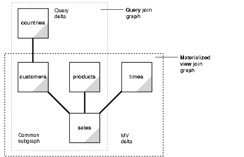
In this check, the joins in a query are compared against the joins in a materialized view. In general, this comparison results in the classification of joins into three categories:
Common joins that occur in both the query and the materialized view. These joins form the common subgraph.
Delta joins that occur in the query but not in the materialized view. These joins form the query delta subgraph.
Delta joins that occur in the materialized view but not in the query. These joins form the materialized view delta subgraph.
These can be visualized as shown in Figure 18-2.
The common join pairs between the two must be of the same type, or the join in the query must be derivable from the join in the materialized view. For example, if a materialized view contains an outer join of table A with table B, and a query contains an inner join of table A with table B, the result of the inner join can be derived by filtering the antijoin rows from the result of the outer join. For example, consider the following query:
SELECT p.prod_name, t.week_ending_day, SUM(amount_sold)
FROM   sales s, products p, times t
WHERE  s.time_id=t.time_id AND s.prod_id = p.prod_id
AND t. week_ending_day BETWEEN TO_DATE('01-AUG-1999', 'DD-MON-YYYY')
                          AND TO_DATE('10-AUG-1999', 'DD-MON-YYYY')
GROUP BY prod_name, week_ending_day;
The common joins between this query and the materialized view join_sales_time_product_mv are:
s.time_id = t.time_id AND s.prod_id = p.prod_id
They match exactly and the query can be rewritten as follows:
SELECT prod_name, week_ending_day, SUM(amount_sold)
FROM   join_sales_time_product_mv
WHERE  week_ending_day BETWEEN TO_DATE('01-AUG-1999','DD-MON-YYYY')
                         AND   TO_DATE('10-AUG-1999','DD-MON-YYYY')
GROUP BY prod_name, week_ending_day;
The query could also be answered using the join_sales_time_product_oj_mv materialized view where inner joins in the query can be derived from outer joins in the materialized view. The rewritten version will (transparently to the user) filter out the antijoin rows. The rewritten query will have the following structure:
SELECT prod_name, week_ending_day, SUM(amount_sold)
FROM   join_sales_time_product_oj_mv
WHERE  week_ending_day BETWEEN TO_DATE('01-AUG-1999','DD-MON-YYYY')
  AND  TO_DATE('10-AUG-1999','DD-MON-YYYY') AND prod_id IS NOT NULL
GROUP BY prod_name, week_ending_day;
In general, if you use an outer join in a materialized view containing only joins, you should put in the materialized view either the primary key or the rowid on the right side of the outer join. For example, in the previous example, join_sales_time_product_oj_mv, there is a primary key on both sales and products.
Another example of when a materialized view containing only joins is used is the case of a semijoin rewrites. That is, a query contains either an EXISTS or an IN subquery with a single table. Consider the following query, which reports the products that had sales greater than $1,000:
SELECT DISTINCT prod_name
FROM products p
WHERE EXISTS (SELECT * FROM sales s
              WHERE p.prod_id=s.prod_id AND s.amount_sold > 1000);
This query could also be represented as:
SELECT DISTINCT prod_name
FROM products p WHERE p.prod_id IN (SELECT s.prod_id FROM sales s
                    WHERE s.amount_sold > 1000);
This query contains a semijoin (s.prod_id = p.prod_id) between the products and the sales table.
This query can be rewritten to use either the join_sales_time_product_mv materialized view, if foreign key constraints are active or join_sales_time_product_oj_mv materialized view, if primary keys are active. Observe that both materialized views contain s.prod_id=p.prod_id, which can be used to derive the semijoin in the query. The query is rewritten with join_sales_time_product_mv as follows:
SELECT prod_name
FROM (SELECT DISTINCT prod_name FROM  join_sales_time_product_mv
      WHERE amount_sold > 1000);
If the materialized view join_sales_time_product_mv is partitioned by time_id, then this query is likely to be more efficient than the original query because the original join between sales and products has been avoided. The query could be rewritten using join_sales_time_product_oj_mv as follows.
SELECT prod_name
FROM (SELECT DISTINCT prod_name FROM  join_sales_time_product_oj_mv
      WHERE amount_sold > 1000 AND prod_id IS NOT NULL);
Rewrites with semi-joins are restricted to materialized views with joins only and are not possible for materialized views with joins and aggregates.
A query delta join is a join that appears in the query but not in the materialized view. Any number and type of delta joins in a query are allowed and they are simply retained when the query is rewritten with a materialized view. In order for the retained join to work, the materialized view must contain the joining key. Upon rewrite, the materialized view is joined to the appropriate tables in the query delta. For example, consider the following query:
SELECT p.prod_name, t.week_ending_day, c.cust_city, SUM(s.amount_sold)
FROM   sales s, products p, times t, customers c
WHERE  s.time_id=t.time_id AND s.prod_id = p.prod_id
AND    s.cust_id = c.cust_id
GROUP BY prod_name, week_ending_day, cust_city;
Using the materialized view join_sales_time_product_mv, common joins are: s.time_id=t.time_id and s.prod_id=p.prod_id. The delta join in the query is s.cust_id=c.cust_id. The rewritten form will then join the join_sales_time_product_mv materialized view with the customers table as follows:
SELECT mv.prod_name, mv.week_ending_day, c.cust_city, SUM(mv.amount_sold)
FROM   join_sales_time_product_mv mv, customers c
WHERE  mv.cust_id = c.cust_id
GROUP BY prod_name, week_ending_day, cust_city;
A materialized view delta join is a join that appears in the materialized view but not the query. All delta joins in a materialized view are required to be lossless with respect to the result of common joins. A lossless join guarantees that the result of common joins is not restricted. A lossless join is one where, if two tables called A and B are joined together, rows in table A will always match with rows in table B and no data will be lost, hence the term lossless join. For example, every row with the foreign key matches a row with a primary key provided no nulls are allowed in the foreign key. Therefore, to guarantee a lossless join, it is necessary to have FOREIGN KEY, PRIMARY KEY, and NOT NULL constraints on appropriate join keys. Alternatively, if the join between tables A and B is an outer join (A being the outer table), it is lossless as it preserves all rows of table A.
All delta joins in a materialized view are required to be non-duplicating with respect to the result of common joins. A non-duplicating join guarantees that the result of common joins is not duplicated. For example, a non-duplicating join is one where, if table A and table B are joined together, rows in table A will match with at most one row in table B and no duplication occurs. To guarantee a non-duplicating join, the key in table B must be constrained to unique values by using a primary key or unique constraint.
Consider the following query that joins sales and times:
SELECT t.week_ending_day, SUM(s.amount_sold)
FROM   sales s, times t
WHERE s.time_id = t.time_id AND t.week_ending_day BETWEEN TO_DATE
 ('01-AUG-1999', 'DD-MON-YYYY') AND TO_DATE('10-AUG-1999', 'DD-MON-YYYY')
GROUP BY week_ending_day;
The materialized view join_sales_time_product_mv has an additional join (s.prod_id=p.prod_id) between sales and products. This is the delta join in join_sales_time_product_mv. You can rewrite the query if this join is lossless and non-duplicating. This is the case if s.prod_id is a foreign key to p.prod_id and is not null. The query is therefore rewritten as:
SELECT week_ending_day, SUM(amount_sold)
FROM   join_sales_time_product_mv
WHERE  week_ending_day BETWEEN TO_DATE('01-AUG-1999', 'DD-MON-YYYY')
                       AND     TO_DATE('10-AUG-1999', 'DD-MON-YYYY')
GROUP BY week_ending_day;
The query can also be rewritten with the materialized view join_sales_time_product_mv_oj where foreign key constraints are not needed. This view contains an outer join (s.prod_id=p.prod_id(+)) between sales and products. This makes the join lossless. If p.prod_id is a primary key, then the non-duplicating condition is satisfied as well and optimizer rewrites the query as follows:
SELECT week_ending_day, SUM(amount_sold)
FROM   join_sales_time_product_oj_mv
WHERE  week_ending_day BETWEEN TO_DATE('01-AUG-1999', 'DD-MON-YYYY')
  AND  TO_DATE('10-AUG-1999', 'DD-MON-YYYY')
GROUP BY week_ending_day;
Note that the outer join in the definition of join_sales_time_product_mv_oj is not necessary because the parent key - foreign key relationship between sales and products in the sh schema is already lossless. It is used for demonstration purposes only, and would be necessary if sales.prod_id were nullable, thus violating the losslessness of the join condition sales.prod_id = products.prod_id.
Current limitations restrict most rewrites with outer joins to materialized views with joins only. There is limited support for rewrites with materialized aggregate views with outer joins, so those views should rely on foreign key constraints to assure losslessness of materialized view delta joins.
Query rewrite is able to make many transformations based upon the recognition of equivalent joins. Query rewrite recognizes the following construct as being equivalent to a join:
WHERE table1.column1 = F(args)   /* sub-expression A */
AND table2.column2 = F(args)     /* sub-expression B */
If F(args) is a PL/SQL function that is declared to be deterministic and the arguments to both invocations of F are the same, then the combination of subexpression A with subexpression B be can be recognized as a join between table1.column1 and table2.column2. That is, the following expression is equivalent to the previous expression:
WHERE table1.column1 = F(args)          /* sub-expression A */
AND table2.column2 = F(args)            /* sub-expression B */
AND table1.column1 = table2.column2     /* join-expression J */
Because join-expression J can be inferred from sub-expression A and subexpression B, the inferred join can be used to match a corresponding join of table1.column1 = table2.column2 in a materialized view.
In this check, the optimizer determines if the necessary column data requested by a query can be obtained from a materialized view. For this, the equivalence of one column with another is used. For example, if an inner join between table A and table B is based on a join predicate A.X = B.X, then the data in column A.X will equal the data in column B.X in the result of the join. This data property is used to match column A.X in a query with column B.X in a materialized view or vice versa. For example, consider the following query:
SELECT p.prod_name, s.time_id, t.week_ending_day, SUM(s.amount_sold)
FROM sales s, products p, times t
WHERE s.time_id=t.time_id AND s.prod_id = p.prod_id
GROUP BY p.prod_name, s.time_id, t.week_ending_day;
This query can be answered with join_sales_time_product_mv even though the materialized view does not have s.time_id. Instead, it has t.time_id, which, through a join condition s.time_id=t.time_id, is equivalent to s.time_id. Thus, the optimizer might select the following rewrite:
SELECT prod_name, time_id, week_ending_day, SUM(amount_sold)
FROM join_sales_time_product_mv
GROUP BY prod_name, time_id, week_ending_day;
This check is required only if both the materialized view and the query contain a GROUP BY clause. The optimizer first determines if the grouping of data requested by a query is exactly the same as the grouping of data stored in a materialized view. In other words, the level of grouping is the same in both the query and the materialized view. If the materialized views groups on all the columns and expressions in the query and also groups on additional columns or expressions, query rewrite can reaggregate the materialized view over the grouping columns and expressions of the query to derive the same result requested by the query.
This check is required only if both the query and the materialized view contain aggregates. Here the optimizer determines if the aggregates requested by a query can be derived or computed from one or more aggregates stored in a materialized view. For example, if a query requests AVG(X) and a materialized view contains SUM(X) and COUNT(X), then AVG(X) can be computed as SUM(X)/COUNT(X).
If the grouping compatibility check determined that the rollup of aggregates stored in a materialized view is required, then the aggregate computability check determines if it is possible to roll up each aggregate requested by the query using aggregates in the materialized view.
The following discusses some of the other cases when query rewrite is possible:
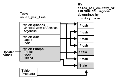
When a partition of the detail table is updated, only specific sections of the materialized view are marked stale. The materialized view must have information that can identify the partition of the table corresponding to a particular row or group of the materialized view. The simplest scenario is when the partitioning key of the table is available in the SELECT list of the materialized view because this is the easiest way to map a row to a stale partition. The key points when using partially stale materialized views are:
Query rewrite can use a materialized view in ENFORCED or TRUSTED mode if the rows from the materialized view used to answer the query are known to be FRESH.
The fresh rows in the materialized view are identified by adding selection predicates to the materialized view's WHERE clause. Oracle will rewrite a query with this materialized view if its answer is contained within this (restricted) materialized view.
The fact table sales is partitioned based on ranges of time_id as follows:
PARTITION BY RANGE (time_id)
(PARTITION SALES_Q1_1998
           VALUES LESS THAN (TO_DATE('01-APR-1998', 'DD-MON-YYYY')),
 PARTITION SALES_Q2_1998
           VALUES LESS THAN (TO_DATE('01-JUL-1998', 'DD-MON-YYYY')),
 PARTITION SALES_Q3_1998
           VALUES LESS THAN (TO_DATE('01-OCT-1998', 'DD-MON-YYYY')),
...
Suppose you have a materialized view grouping by time_id as follows:
CREATE MATERIALIZED VIEW sum_sales_per_city_mv
ENABLE QUERY REWRITE AS
SELECT s.time_id, p.prod_subcategory, c.cust_city,
       SUM(s.amount_sold) AS sum_amount_sold
FROM sales s, products p, customers c
WHERE s.cust_id = c.cust_id AND s.prod_id = p.prod_id
GROUP BY time_id, prod_subcategory, cust_city;
Also suppose new data will be inserted for December 2000, which will be assigned to partition sales_q4_2000. For testing purposes, you can apply an arbitrary DML operation on sales, changing a different partition than sales_q1_2000 as the following query requests data in this partition when this materialized view is fresh. For example, the following:
INSERT INTO SALES VALUES(17, 10, '01-DEC-2000', 4, 380, 123.45, 54321);
Until a refresh is done, the materialized view is generically stale and cannot be used for unlimited rewrite in enforced mode. However, because the table sales is partitioned and not all partitions have been modified, Oracle can identify all partitions that have not been touched. The optimizer can identify the fresh rows in the materialized view (the data which is unaffected by updates since the last refresh operation) by implicitly adding selection predicates to the materialized view defining query as follows:
SELECT s.time_id, p.prod_subcategory, c.cust_city,
       SUM(s.amount_sold) AS sum_amount_sold
FROM sales s, products p, customers c
WHERE s.cust_id = c.cust_id AND s.prod_id = p.prod_id
AND   s.time_id < TO_DATE('01-OCT-2000','DD-MON-YYYY')
OR s.time_id >= TO_DATE('01-OCT-2001','DD-MON-YYYY'))
GROUP BY time_id, prod_subcategory, cust_city;
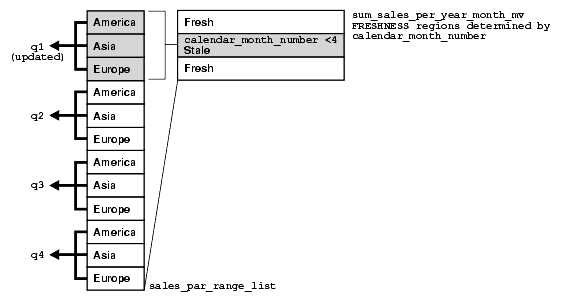
Note that the freshness of partially stale materialized views is tracked on a per-partition base, and not on a logical base. Because the partitioning strategy of the sales fact table is on a quarterly base, changes in December 2000 causes the complete partition sales_q4_2000 to become stale.
Consider the following query, which asks for sales in quarters 1 and 2 of 2000:
SELECT s.time_id, p.prod_subcategory, c.cust_city,
       SUM(s.amount_sold) AS sum_amount_sold
FROM sales s, products p, customers c
WHERE s.cust_id = c.cust_id AND s.prod_id = p.prod_id
AND   s.time_id BETWEEN TO_DATE('01-JAN-2000', 'DD-MON-YYYY')
AND TO_DATE('01-JUL-2000', 'DD-MON-YYYY')
GROUP BY time_id, prod_subcategory, cust_city;
Oracle Database knows that those ranges of rows in the materialized view are fresh and can therefore rewrite the query with the materialized view. The rewritten query looks as follows:
SELECT time_id, prod_subcategory, cust_city, sum_amount_sold
FROM sum_sales_per_city_mv
WHERE time_id BETWEEN TO_DATE('01-JAN-2000', 'DD-MON-YYYY')
AND TO_DATE('01-JUL-2000', 'DD-MON-YYYY');
Instead of the partitioning key, a partition marker (a function that identifies the partition given a rowid) can be present in the select (and GROUP BY list) of the materialized view. You can use the materialized view to rewrite queries that require data from only certain partitions (identifiable by the partition-marker), for instance, queries that have a predicate specifying ranges of the partitioning keys containing entire partitions. See Chapter 9, " Advanced Materialized Views" for details regarding the supplied partition marker function DBMS_MVIEW.PMARKER.
The following example illustrates the use of a partition marker in the materialized view instead of directly using the partition key column:
CREATE MATERIALIZED VIEW sum_sales_per_city_2_mv
ENABLE QUERY REWRITE AS
SELECT DBMS_MVIEW.PMARKER(s.rowid) AS pmarker,
       t.fiscal_quarter_desc, p.prod_subcategory, c.cust_city,
       SUM(s.amount_sold) AS sum_amount_sold
FROM sales s, products p, customers c, times t
WHERE s.cust_id = c.cust_id AND s.prod_id = p.prod_id
AND   s.time_id = t.time_id
GROUP BY DBMS_MVIEW.PMARKER(s.rowid),
    prod_subcategory, cust_city, fiscal_quarter_desc;
Suppose you know that the partition sales_q1_2000 is fresh and DML changes have taken place for other partitions of the sales table. For testing purposes, you can apply an arbitrary DML operation on sales, changing a different partition than sales_q1_2000 when the materialized view is fresh. An example is the following:
INSERT INTO SALES VALUES(17, 10, '01-DEC-2000', 4, 380, 123.45, 54321);
Although the materialized view sum_sales_per_city_2_mv is now considered generically stale, Oracle Database can rewrite the following query using this materialized view. This query restricts the data to the partition sales_q1_2000, and selects only certain values of cust_city, as shown in the following:
SELECT p.prod_subcategory, c.cust_city, SUM(s.amount_sold) AS sum_amount_sold
FROM sales s, products p, customers c, times t
WHERE s.cust_id = c.cust_id AND s.prod_id = p.prod_id AND s.time_id = t.time_id
AND c.cust_city= 'Nuernberg'
AND s.time_id >=TO_DATE('01-JAN-2000','dd-mon-yyyy')
AND s.time_id <  TO_DATE('01-APR-2000','dd-mon-yyyy')
GROUP BY prod_subcategory, cust_city;
Note that rewrite with a partially stale materialized view that contains a PMARKER function can only take place when the complete data content of one or more partitions is accessed and the predicate condition is on the partitioned fact table itself, as shown in the earlier example.
The DBMS_MVIEW.PMARKER function gives you exactly one distinct value for each partition. This dramatically reduces the number of rows in a potential materialized view compared to the partitioning key itself, but you are also giving up any detailed information about this key. The only thing you know is the partition number and, therefore, the lower and upper boundary values. This is the trade-off for reducing the cardinality of the range partitioning column and thus the number of rows.
Assuming the value of p_marker for partition sales_q1_2000 is 31070, the previously shown queries can be rewritten against the materialized view as follows:
SELECT mv.prod_subcategory, mv.cust_city, SUM(mv.sum_amount_sold)
FROM sum_sales_per_city_2_mv mv
WHERE mv.pmarker = 31070 AND mv.cust_city= 'Nuernberg'
GROUP BY prod_subcategory, cust_city;
So the query can be rewritten against the materialized view without accessing stale data.
Query rewrite attempts to iteratively take advantage of nested materialized views. Oracle Database first tries to rewrite a query with materialized views having aggregates and joins, then with a materialized view containing only joins. If any of the rewrites succeeds, Oracle repeats that process again until no rewrites are found. For example, assume that you had created materialized views join_sales_time_product_mv and sum_sales_time_product_mv as in the following:
CREATE MATERIALIZED VIEW join_sales_time_product_mv
ENABLE QUERY REWRITE AS
SELECT p.prod_id, p.prod_name, t.time_id, t.week_ending_day,
       s.channel_id, s.promo_id, s.cust_id, s.amount_sold
FROM   sales s, products p, times t
WHERE  s.time_id=t.time_id AND s.prod_id = p.prod_id;

CREATE MATERIALIZED VIEW sum_sales_time_product_mv
ENABLE QUERY REWRITE AS
SELECT mv.prod_name, mv.week_ending_day, COUNT(*) cnt_all,
       SUM(mv.amount_sold) sum_amount_sold,
       COUNT(mv.amount_sold) cnt_amount_sold
FROM join_sales_time_product_mv mv
GROUP BY mv.prod_name, mv.week_ending_day;
Then consider the following query:
SELECT p.prod_name, t.week_ending_day, SUM(s.amount_sold)
FROM sales s, products p, times t
WHERE s.time_id=t.time_id AND s.prod_id=p.prod_id
GROUP BY p.prod_name, t.week_ending_day;
Oracle first tries to rewrite it with a materialized aggregate view and finds there is none eligible (note that single-table aggregate materialized view sum_sales_store_time_mv cannot yet be used), and then tries a rewrite with a materialized join view and finds that join_sales_time_product_mv is eligible for rewrite. The rewritten query has this form:
SELECT mv.prod_name, mv.week_ending_day, SUM(mv.amount_sold)
FROM join_sales_time_product_mv mv
GROUP BY mv.prod_name, mv.week_ending_day;
Because a rewrite occurred, Oracle tries the process again. This time, the query can be rewritten with single-table aggregate materialized view sum_sales_store_time into the following form:
SELECT mv.prod_name, mv.week_ending_day, mv.sum_amount_sold
FROM sum_sales_time_product_mv mv;
Several extensions to the GROUP BY clause in the form of GROUPING SETS, CUBE, ROLLUP, and their concatenation are available. These extensions enable you to selectively specify the groupings of interest in the GROUP BY clause of the query. For example, the following is a typical query with grouping sets:
SELECT p.prod_subcategory, t.calendar_month_desc, c.cust_city,
  SUM(s.amount_sold) AS sum_amount_sold
FROM sales s, customers c, products p, times t
WHERE s.time_id=t.time_id AND s.prod_id = p.prod_id AND s.cust_id = c.cust_id
GROUP BY GROUPING SETS ((p.prod_subcategory, t.calendar_month_desc),
   (c.cust_city, p.prod_subcategory));
The term base grouping for queries with GROUP BY extensions denotes all unique expressions present in the GROUP BY clause. In the previous query, the following grouping (p.prod_subcategory, t.calendar_month_desc, c.cust_city) is a base grouping.
The extensions can be present in user queries and in the queries defining materialized views. In both cases, materialized view rewrite applies and you can distinguish rewrite capabilities into the following scenarios:
Materialized View has Simple GROUP BY and Query has Extended GROUP BY
Materialized View has Extended GROUP BY and Query has Simple GROUP BY
When a query contains an extended GROUP BY clause, it can be rewritten with a materialized view if its base grouping can be rewritten using the materialized view as listed in the rewrite rules explained in "When Does Oracle Rewrite a Query?". For example, in the following query:
SELECT p.prod_subcategory, t.calendar_month_desc, c.cust_city,
  SUM(s.amount_sold) AS sum_amount_sold
FROM sales s, customers c, products p, times t
WHERE s.time_id=t.time_id AND s.prod_id = p.prod_id AND s.cust_id = c.cust_id
GROUP BY GROUPING SETS
((p.prod_subcategory, t.calendar_month_desc),
   (c.cust_city, p.prod_subcategory));
The base grouping is (p.prod_subcategory, t.calendar_month_desc, c.cust_city, p.prod_subcategory)) and, consequently, Oracle can rewrite the query using sum_sales_pscat_month_city_mv as follows:
SELECT mv.prod_subcategory, mv.calendar_month_desc, mv.cust_city,
  SUM(mv.sum_amount_sold) AS sum_amount_sold
FROM sum_sales_pscat_month_city_mv mv
GROUP BY GROUPING SETS
((mv.prod_subcategory, mv.calendar_month_desc),
  (mv.cust_city, mv.prod_subcategory));
A special situation arises if the query uses the EXPAND_GSET_TO_UNION hint. See "Hint for Queries with Extended GROUP BY" for an example of using EXPAND_GSET_TO_UNION.
In order for a materialized view with an extended GROUP BY to be used for rewrite, it must satisfy two additional conditions:
It must contain a grouping distinguisher, which is the GROUPING_ID function on all GROUP BY expressions. For example, if the GROUP BY clause of the materialized view is GROUP BY CUBE(a, b), then the SELECT list should contain GROUPING_ID(a, b).
The GROUP BY clause of the materialized view should not result in any duplicate groupings. For example, GROUP BY GROUPING SETS ((a, b), (a, b)) would disqualify a materialized view from general rewrite.
A materialized view with an extended GROUP BY contains multiple groupings. Oracle finds the grouping with the lowest cost from which the query can be computed and uses that for rewrite. For example, consider the following materialized view:
CREATE MATERIALIZED VIEW sum_grouping_set_mv
ENABLE QUERY REWRITE AS
SELECT p.prod_category, p.prod_subcategory, c.cust_state_province, c.cust_city,
  GROUPING_ID(p.prod_category,p.prod_subcategory,
              c.cust_state_province,c.cust_city) AS gid,
  SUM(s.amount_sold) AS sum_amount_sold
FROM sales s, products p, customers c
WHERE s.prod_id = p.prod_id AND s.cust_id = c.cust_id
GROUP BY GROUPING SETS
((p.prod_category, p.prod_subcategory, c.cust_city),
  (p.prod_category, p.prod_subcategory, c.cust_state_province, c.cust_city),
  (p.prod_category, p.prod_subcategory));
In this case, the following query will be rewritten:
SELECT p.prod_subcategory, c.cust_city, SUM(s.amount_sold) AS sum_amount_sold
FROM sales s, products p, customers c
WHERE s.prod_id = p.prod_id AND s.cust_id = c.cust_id
GROUP BY p.prod_subcategory, c.cust_city;
This query will be rewritten with the closest matching grouping from the materialized view. That is, the (prodcategory, prod_subcategory, cust_city) grouping:
SELECT prod_subcategory, cust_city, SUM(sum_amount_sold) AS sum_amount_sold
FROM sum_grouping_set_mv
WHERE gid = grouping identifier of (prod_category,prod_subcategory, cust_city)
GROUP BY prod_subcategory, cust_city;
When both materialized view and the query contain GROUP BY extensions, Oracle uses two strategies for rewrite: grouping match and UNION ALL rewrite. First, Oracle tries grouping match. The groupings in the query are matched against groupings in the materialized view and if all are matched with no rollup, Oracle selects them from the materialized view. For example, consider the following query:
SELECT p.prod_category, p.prod_subcategory, c.cust_city,
       SUM(s.amount_sold) AS sum_amount_sold
FROM sales s, products p, customers c
WHERE s.prod_id = p.prod_id AND s.cust_id = c.cust_id
GROUP BY GROUPING SETS
((p.prod_category, p.prod_subcategory, c.cust_city),
  (p.prod_category, p.prod_subcategory));
This query matches two groupings from sum_grouping_set_mv and Oracle rewrites the query as the following:
SELECT prod_subcategory, cust_city, sum_amount_sold
FROM sum_grouping_set_mv
WHERE gid = grouping identifier of (prod_category,prod_subcategory, cust_city)
   OR gid = grouping identifier of (prod_category,prod_subcategory)
If grouping match fails, Oracle tries a general rewrite mechanism called UNION ALL rewrite. Oracle first represents the query with the extended GROUP BY clause as an equivalent UNION ALL query. Every grouping of the original query is placed in a separate UNION ALL branch. The branch will have a simple GROUP BY clause. For example, consider this query:
SELECT p.prod_category, p.prod_subcategory, c.cust_state_province,
  t.calendar_month_desc, SUM(s.amount_sold) AS sum_amount_sold
FROM sales s, products p, customers c, times t
WHERE s.prod_id = p.prod_id AND s.cust_id = c.cust_id
GROUP BY GROUPING SETS
((p.prod_subcategory, t.calendar_month_desc),
  (t.calendar_month_desc),
  (p.prod_category, p.prod_subcategory, c.cust_state_province),
  (p.prod_category, p.prod_subcategory));
This is first represented as UNION ALL with four branches:
SELECT null, p.prod_subcategory, null,
    t.calendar_month_desc, SUM(s.amount_sold) AS sum_amount_sold
FROM sales s, products p, customers c, times t
WHERE s.prod_id = p.prod_id AND s.cust_id = c.cust_id
GROUP BY p.prod_subcategory, t.calendar_month_desc
UNION ALL
  SELECT null, null, null,
    t.calendar_month_desc, SUM(s.amount_sold) AS sum_amount_sold
FROM sales s, products p, customers c, times t
WHERE s.prod_id = p.prod_id AND s.cust_id = c.cust_id
GROUP BY t.calendar_month_desc
UNION ALL
SELECT p.prod_category, p.prod_subcategory, c.cust_state_province,
    null, SUM(s.amount_sold) AS sum_amount_sold
FROM sales s, products p, customers c, times t
WHERE s.prod_id = p.prod_id AND s.cust_id = c.cust_id
GROUP BY p.prod_category, p.prod_subcategory, c.cust_state_province
UNION ALL
  SELECT p.prod_category, p.prod_subcategory, null,
    null, SUM(s.amount_sold) AS sum_amount_sold
  FROM sales s, products p, customers c, times t
  WHERE s.prod_id = p.prod_id AND s.cust_id = c.cust_id
  GROUP BY p.prod_category, p.prod_subcategory;
Each branch is then rewritten separately using the rules from "When Does Oracle Rewrite a Query?". Using the materialized view sum_grouping_set_mv, Oracle can rewrite only branches three (which requires materialized view rollup) and four (which matches the materialized view exactly). The unrewritten branches will be converted back to the extended GROUP BY form. Thus, eventually, the query is rewritten as:
SELECT null, p.prod_subcategory, null,
    t.calendar_month_desc, SUM(s.amount_sold) AS sum_amount_sold
FROM sales s, products p, customers c, times t
WHERE s.prod_id = p.prod_id AND s.cust_id = c.cust_id
GROUP BY GROUPING SETS
  ((p.prod_subcategory, t.calendar_month_desc),
    (t.calendar_month_desc),)
UNION ALL
  SELECT prod_category, prod_subcategory, cust_state_province,
    null, SUM(sum_amount_sold) AS sum_amount_sold
  FROM sum_grouping_set_mv
  WHERE gid = <grouping id of (prod_category,prod_subcategory, cust_city)>
  GROUP BY p.prod_category, p.prod_subcategory, c.cust_state_province
UNION ALL
  SELECT prod_category, prod_subcategory, null,
    null, sum_amount_sold
  FROM sum_grouping_set_mv
  WHERE gid = <grouping id of (prod_category,prod_subcategory)>
Note that a query with extended GROUP BY is represented as an equivalent UNION ALL and recursively submitted for rewrite optimization. The groupings that cannot be rewritten stay in the last branch of UNION ALL and access the base data instead.
You can use the EXPAND_GSET_TO_UNION hint to force expansion of the query with GROUP BY extensions into the equivalent UNION ALL query. This hint can be used in an environment where materialized views have simple GROUP BY clauses only. In this case, Oracle extends rewrite flexibility as each branch can be independently rewritten by a separate materialized view. See Oracle Database Performance Tuning Guide for more information regarding EXPAND_GSET_TO_UNION
Oracle Database supports general query rewrite when the user query contains an inline view, or a subquery in the FROM list. Query rewrite matches inline views in the materialized view with inline views in the request query when the text of the two inline views exactly match. In this case, rewrite treats the matching inline view as it would a named view, and general rewrite processing is possible.
The following is an example where the materialized view contains an inline view, and the query has the same inline view, but the aliases for these views are different:
CREATE MATERIALIZED VIEW inline_example
ENABLE QUERY REWRITE AS
SELECT t.calendar_month_name, t.calendar_year  p.prod_category,
       SUM(V1.revenue) AS sum_revenue
FROM times t, products p,
     (SELECT time_id, prod_id, amount_sold*0.2 AS revenue FROM sales) V1
WHERE t.time_id = V1.time_id AND p.prod_id = V1.prod_id
GROUP BY calendar_month_name, calendar_year, prod_category;
And here is the query that will be rewritten to use the materialized view:
SELECT t.calendar_month_name, t.calendar_year, p.prod_category,
       SUM(X1.revenue) AS sum_revenue
FROM times t, products p,
     (SELECT time_id, prod_id, amount_sold*0.2 AS revenue FROM sales) X1
WHERE t.time_id = X1.time_id AND p.prod_id = X1.prod_id
GROUP BY calendar_month_name, calendar_year, prod_category;
Oracle accomplishes query rewrite of queries which contain multiple references to the same tables, or self joins by employing two different strategies. Using the first strategy, you need to ensure that the query and the materialized view definitions have the same aliases for the multiple references to a table. If you do not provide a matching alias, Oracle will try the second strategy, where the joins in the query and the materialized view are compared to match the multiple references in the query to the multiple references in the materialized view.
The following is an example of a materialized view and a query. In this example, the query is missing a reference to a column in a table so an exact text match will not work. General query rewrite can occur, however, because the aliases for the table references match.
To demonstrate the self-join rewriting possibility with the sh sample schema, the following addition is assumed to include the actual shipping and payment date in the fact table, referencing the same dimension table times. This is for demonstration purposes only and will not return any results:
ALTER TABLE sales ADD (time_id_ship DATE);
ALTER TABLE sales ADD (CONSTRAINT time_id_book_fk FOREIGN key (time_id_ship)
REFERENCES times(time_id) ENABLE NOVALIDATE);
ALTER TABLE sales MODIFY CONSTRAINT time_id_book_fk RELY;
ALTER TABLE sales ADD (time_id_paid DATE);
ALTER TABLE sales ADD (CONSTRAINT time_id_paid_fk FOREIGN KEY (time_id_paid)
REFERENCES times(time_id) ENABLE NOVALIDATE);
ALTER TABLE sales MODIFY CONSTRAINT time_id_paid_fk RELY;
Now, you can define a materialized view as follows:
CREATE MATERIALIZED VIEW sales_shipping_lag_mv
ENABLE QUERY REWRITE AS
SELECT t1.fiscal_week_number, s.prod_id,
         t2.fiscal_week_number - t1.fiscal_week_number as lag
FROM times t1, sales s, times t2
WHERE t1.time_id = s.time_id AND t2.time_id = s.time_id_ship;
The following query fails the exact text match test but is rewritten because the aliases for the table references match:
SELECT s.prod_id, t2.fiscal_week_number - t1.fiscal_week_number AS lag
FROM times t1, sales s, times t2
WHERE t1.time_id = s.time_id AND t2.time_id = s.time_id_ship;
Note that Oracle performs other checks to ensure the correct match of an instance of a multiply instanced table in the request query with the corresponding table instance in the materialized view. For instance, in the following example, Oracle correctly determines that the matching alias names used for the multiple instances of table time does not establish a match between the multiple instances of table time in the materialized view.
The following query cannot be rewritten using sales_shipping_lag_mv, even though the alias names of the multiply instanced table time match because the joins are not compatible between the instances of time aliased by t2:
SELECT s.prod_id, t2.fiscal_week_number - t1.fiscal_week_number AS lag
FROM times t1, sales s, times t2
WHERE t1.time_id = s.time_id AND t2.time_id = s.time_id_paid;
This request query joins the instance of the time table aliased by t2 on the s.time_id_paid column, while the materialized views joins the instance of the time table aliased by t2 on the s.time_id_ship column. Because the join conditions differ, Oracle correctly determines that rewrite cannot occur.
The following query does not have any matching alias in the materialized view, sales_shipping_lag_mv, for the table, times. But query rewrite will now compare the joins between the query and the materialized view and correctly match the multiple instances of times.
SELECT s.prod_id, x2.fiscal_week_number - x1.fiscal_week_number AS lag
FROM times x1, sales s, times x2
WHERE x1.time_id = s.time_id AND x2.time_id = s.time_id_ship;
Data warehouse applications recognize multi-dimensional cubes in the database by identifying integrity constraints in the relational schema. Integrity constraints represent primary and foreign key relationships between fact and dimension tables. By querying the data dictionary, applications can recognize integrity constraints and hence the cubes in the database. However, this does not work in an environment where database administrators, for schema complexity or security reasons, define views on fact and dimension tables. In such environments, applications cannot identify the cubes properly. By allowing constraint definitions between views, you can propagate base table constraints to the views, thereby allowing applications to recognize cubes even in a restricted environment.
View constraint definitions are declarative in nature, but operations on views are subject to the integrity constraints defined on the underlying base tables, and constraints on views can be enforced through constraints on base tables. Defining constraints on base tables is necessary, not only for data correctness and cleanliness, but also for materialized view query rewrite purposes using the original base objects.
Materialized view rewrite extensively uses constraints for query rewrite. They are used for determining lossless joins, which, in turn, determine if joins in the materialized view are compatible with joins in the query and thus if rewrite is possible.
DISABLE NOVALIDATE is the only valid state for a view constraint. However, you can choose RELY or NORELY as the view constraint state to enable more sophisticated query rewrites. For example, a view constraint in the RELY state allows query rewrite to occur when the query integrity level is set to TRUSTED. Table 18-2 illustrates when view constraints are used for determining lossless joins.
Note that view constraints cannot be used for query rewrite integrity level ENFORCED. This level enforces the highest degree of constraint enforcement ENABLE VALIDATE.
Table 18-2 View Constraints and Rewrite Integrity Modes
| Constraint States | RELY | NORELY |
|---|---|---|
ENFORCED |
No | No |
TRUSTED |
Yes | No |
STALE_TOLERATED |
Yes | No |
Example 18-10 View Constraints
To demonstrate the rewrite capabilities on views, you need to extend the sh sample schema as follows:
CREATE VIEW time_view AS
SELECT time_id, TO_NUMBER(TO_CHAR(time_id, 'ddd')) AS day_in_year FROM times;
You can now establish a foreign key/primary key relationship (in RELY ON) mode between the view and the fact table, and thus rewrite will take place as described in Table 18-2, by adding the following constraints. Rewrite will then work for example in TRUSTED mode.
ALTER VIEW time_view ADD (CONSTRAINT time_view_pk
   PRIMARY KEY (time_id) DISABLE NOVALIDATE);
ALTER VIEW time_view MODIFY CONSTRAINT time_view_pk RELY;
ALTER TABLE sales ADD (CONSTRAINT time_view_fk FOREIGN KEY (time_id)
   REFERENCES time_view(time_id) DISABLE NOVALIDATE);
ALTER TABLE sales MODIFY CONSTRAINT time_view_fk RELY;
Consider the following materialized view definition:
CREATE MATERIALIZED VIEW sales_pcat_cal_day_mv
ENABLE QUERY REWRITE AS
SELECT p.prod_category, t.day_in_year, SUM(s.amount_sold) AS sum_amount_sold
FROM time_view t, sales s, products p
WHERE t.time_id = s.time_id AND p.prod_id = s.prod_id
GROUP BY p.prod_category, t.day_in_year;
The following query, omitting the dimension table products, will also be rewritten without the primary key/foreign key relationships, because the suppressed join between sales and products is known to be lossless.
SELECT t.day_in_year, SUM(s.amount_sold) AS sum_amount_sold
FROM time_view t, sales s WHERE t.time_id = s.time_id
GROUP BY t.day_in_year;
However, if the materialized view sales_pcat_cal_day_mv were defined only in terms of the view time_view, then you could not rewrite the following query, suppressing then join between sales and time_view, because there is no basis for losslessness of the delta materialized view join. With the additional constraints as shown previously, this query will also rewrite.
SELECT p.prod_category, SUM(s.amount_sold) AS sum_amount_sold
FROM sales s, products p WHERE p.prod_id = s.prod_id
GROUP BY p.prod_category;
To undo the changes you have made to the sh schema, issue the following statements:
ALTER TABLE sales DROP CONSTRAINT time_view_fk;
DROP VIEW time_view;
If the referential constraint definition involves a view, that is, either the foreign key or the referenced key resides in a view, the constraint can only be in DISABLE NOVALIDATE mode.
A RELY constraint on a view is allowed only if the referenced UNIQUE or PRIMARY KEY constraint in DISABLE NOVALIDATE mode is also a RELY constraint.
The specification of ON DELETE actions associated with a referential Integrity constraint, is not allowed (for example, DELETE cascade). However, DELETE, UPDATE, and INSERT operations are allowed on views and their base tables as view constraints are in DISABLE NOVALIDATE mode.
An expression that appears in a query can be replaced with a simple column in a materialized view provided the materialized view column represents a precomputed expression that matches with the expression in the query. If a query can be rewritten to use a materialized view, it will be faster. This is because materialized views contain precomputed calculations and do not need to perform expression computation.
The expression matching is done by first converting the expressions into canonical forms and then comparing them for equality. Therefore, two different expressions will generally be matched as long as they are equivalent to each other. Further, if the entire expression in a query fails to match with an expression in a materialized view, then subexpressions of it are tried to find a match. The subexpressions are tried in a top-down order to get maximal expression matching.
Consider a query that asks for sum of sales by age brackets (1-10, 11-20, 21-30, and so on).
CREATE MATERIALIZED VIEW sales_by_age_bracket_mv
ENABLE QUERY REWRITE AS
SELECT TO_CHAR((2000-c.cust_year_of_birth)/10-0.5,999) AS age_bracket,
       SUM(s.amount_sold) AS sum_amount_sold
FROM sales s, customers c WHERE s.cust_id=c.cust_id
GROUP BY TO_CHAR((2000-c.cust_year_of_birth)/10-0.5,999);
The following query rewrites, using expression matching:
SELECT TO_CHAR(((2000-c.cust_year_of_birth)/10)-0.5,999), SUM(s.amount_sold)
FROM sales s, customers c WHERE s.cust_id=c.cust_id
GROUP BY TO_CHAR((2000-c.cust_year_of_birth)/10-0.5,999);
This query is rewritten in terms of sum_sales_mv based on the matching of the canonical forms of the age bracket expressions (that is, 2000 - c.cust_year_of_birth)/10-0.5), as follows:
SELECT age_bracket, sum_amount_sold FROM sales_by_age_bracket_mv;
Date folding rewrite is a specific form of expression matching rewrite. In this type of rewrite, a date range in a query is folded into an equivalent date range representing higher date granules. The resulting expressions representing higher date granules in the folded date range are matched with equivalent expressions in a materialized view. The folding of date range into higher date granules such as months, quarters, or years is done when the underlying datatype of the column is an Oracle DATE. The expression matching is done based on the use of canonical forms for the expressions.
DATE is a built-in datatype which represents ordered time units such as seconds, days, and months, and incorporates a time hierarchy (second -> minute -> hour -> day -> month -> quarter -> year). This hard-coded knowledge about DATE is used in folding date ranges from lower-date granules to higher-date granules. Specifically, folding a date value to the beginning of a month, quarter, year, or to the end of a month, quarter, year is supported. For example, the date value 1-jan-1999 can be folded into the beginning of either year 1999 or quarter 1999-1 or month 1999-01. And, the date value 30-sep-1999 can be folded into the end of either quarter 1999-03 or month 1999-09.
|
Note: Due to the way date folding works, you should be careful when usingBETWEEN and date columns. The best way to use BETWEEN and date columns is to increment the later date by 1. In other words, instead of using date_col BETWEEN '1-jan-1999' AND '30-jun-1999', you should use date_col BETWEEN '1-jan-1999' AND '1-jul-1999'. You could also use the TRUNC function to get the equivalent result, as in TRUNC(date_col) BETWEEN '1-jan-1999' AND '30-jun-1999'. TRUNC will, however, strip time values. |
Because date values are ordered, any range predicate specified on date columns can be folded from lower level granules into higher level granules provided the date range represents an integral number of higher level granules. For example, the range predicate date_col >= '1-jan-1999' AND date_col < '30-jun-1999' can be folded into either a month range or a quarter range using the TO_CHAR function, which extracts specific date components from a date value.
The advantage of aggregating data by folded date values is the compression of data achieved. Without date folding, the data is aggregated at the lowest granularity level, resulting in increased disk space for storage and increased I/O to scan the materialized view.
Consider a query that asks for the sum of sales by product types for the years 1998.
SELECT p.prod_category, SUM(s.amount_sold)
FROM sales s, products p
WHERE s.prod_id=p.prod_id AND s.time_id >= TO_DATE('01-jan-1998', 'dd-mon-yyyy')
  AND s.time_id <   TO_DATE('01-jan-1999', 'dd-mon-yyyy')
GROUP BY p.prod_category;

CREATE MATERIALIZED VIEW sum_sales_pcat_monthly_mv
ENABLE QUERY REWRITE AS
SELECT p.prod_category, TO_CHAR(s.time_id,'YYYY-MM') AS month,
       SUM(s.amount_sold) AS sum_amount
FROM sales s, products p
WHERE s.prod_id=p.prod_id
GROUP BY p.prod_category, TO_CHAR(s.time_id, 'YYYY-MM');

SELECT p.prod_category, SUM(s.amount_sold)
FROM sales s, products p
WHERE s.prod_id=p.prod_id
AND TO_CHAR(s.time_id, 'YYYY-MM') >= '01-jan-1998'
AND TO_CHAR(s.time_id, 'YYYY-MM') < '01-jan-1999'
GROUP BY p.prod_category;

SELECT mv.prod_category, mv.sum_amount
FROM sum_sales_pcat_monthly_mv mv
WHERE month >= '01-jan-1998' AND month < '01-jan-1999';
The range specified in the query represents an integral number of years, quarters, or months. Assume that there is a materialized view mv3 that contains pre-summarized sales by prod_type and is defined as follows:
CREATE MATERIALIZED VIEW mv3
ENABLE QUERY REWRITE AS
SELECT prod_type, TO_CHAR(sale_date,'yyyy-mm') AS month, SUM(sales) AS sum_sales
FROM sales, products WHERE sales.prod_id = products.prod_id
GROUP BY prod_type, TO_CHAR(sale_date, 'yyyy-mm');
The query can be rewritten by first folding the date range into the month range and then matching the expressions representing the months with the month expression in mv3. This rewrite is shown in two steps (first folding the date range followed by the actual rewrite).
SELECT prod_type, SUM(sales) AS sum_sales
FROM sales, products
WHERE sales.prod_id = products.prod_id AND TO_CHAR(sale_date, 'yyyy-mm') >=
      TO_CHAR('01-jan-1998', 'yyyy-mm') AND TO_CHAR('01-jan-1999', 'yyyy-mm')
GROUP BY prod_type;

SELECT prod_type, sum_sales
FROM mv3 WHERE month >=
      TO_CHAR('01-jan-1998', 'yyyy-mm')
  AND month < TO_CHAR('01-jan-1999', 'yyyy-mm');
GROUP BY prod_type;
If mv3 had pre-summarized sales by prod_type and year instead of prod_type and month, the query could still be rewritten by folding the date range into year range and then matching the year expressions.
PCT rewrite enables the optimizer to accurately rewrite queries with fresh data using materialized views that are only partially fresh. To do so, Oracle keeps track of which partitions in the detail tables have been updated. Oracle then tracks which rows in the materialized view originate from the affected partitions in the detail tables. The optimizer is then able to use those portions of the materialized view that are known to be fresh.
The optimizer uses PCT rewrite in QUERY_REWRITE_INTEGRITY = ENFORCED and TRUSTED modes. The optimizer does not use PCT rewrite in STALE_TOLERATED mode because data freshness is not considered in that mode.
You can use PCT rewrite with partitioning, but hash partitioning is not supported. The following sections discuss aspects of using PCT:
If the LIST partitioning key is present in the materialized view's SELECT and GROUP BY, then PCT will be supported by the materialized view. Regardless of the supported partitioning type, if the partition marker or rowid of the detail table is present in the materialized view then PCT is supported by the materialized view on that specific detail table.
CREATE TABLE sales_par_list
(calendar_year, calendar_month_number, day_number_in_month,
 country_name, prod_id, quantity_sold, amount_sold)
 PARTITION BY LIST (country_name)
 (PARTITION America
      VALUES ('United States of America', 'Argentina'),
  PARTITION Asia
      VALUES ('Japan', 'India'),
  PARTITION Europe
      VALUES ('France', 'Spain', 'Ireland'))
  AS SELECT t.calendar_year, t.calendar_month_number,
         t.day_number_in_month, c1.country_name, s.prod_id,
         s.quantity_sold, s.amount_sold
  FROM times t, countries c1, sales s, customers c2
  WHERE s.time_id = t.time_id and s.cust_id = c2.cust_id and
        c2.country_id = c1.country_id and
        c1.country_name IN ('United States of America', 'Argentina',
       'Japan', 'India', 'France', 'Spain', 'Ireland');
If a materialized view is created on the table sales_par_list, which has a list partitioning key, PCT rewrite will use that materialized view for potential rewrites.
To illustrate this feature, the following example creates a materialized view that has the total amounts sold of every product in each country for each year. The view depends on detail tables sales_par_list and product.
CREATE MATERIALIZED VIEW sales_per_country_mv
BUILD IMMEDIATE
REFRESH FORCE ON DEMAND
ENABLE QUERY REWRITE AS
SELECT s.calendar_year calendar_year, s.country_name country_name,
 p.prod_name prod_name, SUM(s.amount_sold) AS sum_sales, COUNT(*) AS cnt
FROM sales_par_list s, products p
WHERE s.prod_id = p.prod_id AND s.calendar_year <= 2000
GROUP BY s.calendar_year, s.country_name, prod_name;
sales_per_country_mv supports PCT against sales_par_list as its list partition key country_name is in its SELECT and GROUP BY list. Table products is not partitioned, so sales_per_country_mv does not support PCT against this table.
A query could be rewritten (in ENFORCED or TRUSTED modes) in terms of sales_per_country_mv even if sales_per_country_mv is stale if the incoming query accesses only fresh parts of the materialized view. You can determine which parts of the materialized view are FRESH only if the updated tables are PCT enabled in the materialized view; if non-PCT enabled tables have been updated then the rewrite is not possible with fresh data from that specific materialized view as you cannot identify the FRESH portions of the materialized view.
sales_per_country_mv supports PCT on sales_par_list and does not support PCT on table product. If table product is updated, then PCT rewrite is not possible with sales_per_country_mv as you cannot tell which portions of the materialized view are FRESH.
The following updates sales_par_list as follows:
INSERT INTO sales_par_list VALUES (2000, 10, 22, 'France', 900, 20, 200.99);
This statement inserted a row into partition Europe in table sales_par_list. Now sales_per_country_mv is stale, but PCT rewrite (in ENFORCED and TRUSTED modes) is possible as this materialized view supports PCT against table sales_par_list. The fresh and stale areas of the materialized view are identified based on the partitioned detail table sales_par_list.
Figure 18-3 illustrates what is fresh and what is stale in this example.
Consider the following query:
SELECT s.country_name, p.prod_name, SUM(s.amount_sold) AS sum_sales,
   COUNT(*) AS cnt
FROM sales_par_list s, products p
WHERE s.prod_id = p.prod_id AND s.calendar_year = 2000 AND
   s.country_name IN ('United States of America', 'Japan')
GROUP BY s.country_name, p.prod_name;
This query accesses partitions America and Asia in sales_par_list; these partition have not been updated so rewrite is possible with stale materialized view sales_per_country_mv as this query will access only FRESH portions of the materialized view.
The query is rewritten in terms of sales_per_country_mv as follows:
SELECT country_name, prod_name, SUM(sum_sales) AS sum_slaes, SUM(cnt) AS cnt
FROM sales_per_country_mv WHERE calendar_year = 2000
  AND country_name IN ('United States of America', 'Japan')
GROUP BY country_name, prod_name;
Now consider the following query:
SELECT s.country_name,  p.prod_name,
 SUM(s.amount_sold) AS sum_sales, COUNT(*) AS cnt
FROM sales_par_list s, products p
WHERE  s.prod_id = p.prod_id AND s.calendar_year = 1999 AND
       s.country_name IN ('Japan', 'India', 'Spain')
GROUP BY s.country_name, p.prod_name;
This query accesses partitions Europe and Asia in sales_par_list; partition Europe has been updated so this query cannot be rewritten in terms of sales_per_country_mv as the required data from the materialized view is stale.
You will be able to rewrite after any kinds of updates to sales_par_list, that is DMLs, direct loads and Partition Maintenance Operations (PMOPs) if the incoming query accesses FRESH parts of the materialized view.
When a partition marker is provided, the query rewrite capabilities are limited to rewrite queries that access whole detail table partitions as all rows from a specific partition have the same pmarker value. That is, if a query accesses a portion of a detail table partition, it is not rewritten even if that data corresponds to a FRESH portion of the materialized view. Now FRESH portions of the materialized view are determined by the pmarker value. To determine which rows of the materialized view are fresh, you associate freshness with the marker value, so all rows in the materialized view with a specific pmarker value are FRESH or are STALE.
The following creates a materialized view has the total amounts sold of every product in each detail table partition of sales_par_list for each year. This materialized view will also depend on detail table products as shown in the following:
CREATE MATERIALIZED VIEW sales_per_dt_partition_mv
BUILD IMMEDIATE
REFRESH FORCE ON DEMAND
ENABLE QUERY REWRITE AS
SELECT s.calendar_year calendar_year, p.prod_name prod_name,
       DBMS_MVIEW.PMARKER(s.rowid) pmarker,
       SUM(s.amount_sold) AS sum_sales, COUNT(*) AS cnt
FROM sales_par_list s, products p
WHERE s.prod_id = p.prod_id AND s.calendar_year > 2000
GROUP BY s.calendar_year, DBMS_MVIEW.PMARKER(s.rowid), p.prod_name;
The materialized view sales_per_dt_partition_mv provides the sum of sales for each detail table partition. This materialized view supports PCT rewrite against table sales_par_list because the partition marker is in its SELECT and GROUP BY clauses. Table 18-3 lists the partition names and their pmarkers for this example.
Table 18-3 Partition Names and Their Pmarkers
| Partition Name | Pmarker |
|---|---|
| America | 1000 |
| Asia | 1001 |
| Europe | 1002 |
Then update the table sales_par_list as follows:
DELETE FROM sales_par_list WHERE country_name = 'India';
You have deleted rows from partition Asia in table sales_par_list. Now sales_per_dt_partition_mv is stale, but PCT rewrite (in ENFORCED and TRUSTED modes) is possible as this materialized view supports PCT (pmarker based) against table sales_par_list.
Now consider the following query:
SELECT p.prod_name, SUM(s.amount_sold) AS sum_sales, COUNT(*) AS cnt
FROM sales_par_list s, products p
WHERE  s.prod_id = p.prod_id AND s.calendar_year = 2001 AND
       s.country_name IN ('United States of America', 'Argentina')
GROUP BY p.prod_name;
This query can be rewritten in terms of sales_per_dt_partition_mv as all the data corresponding to a detail table partition is accessed, and the materialized view is FRESH with respect to this data. This query accesses all data in partition America, which has not been updated.
The query is rewritten in terms of sales_per_dt_partition_mv as follows:
SELECT prod_name, SUM(sum_sales) AS sum_sales, SUM(cnt) AS cnt
FROM sales_per_dt_partition_mv
WHERE calendar_year = 2001 AND pmarker = 1000
GROUP BY prod_name;
If the detail table is range-list partitioned, a materialized view that depends on this detail table can support PCT at both the partitioning and subpartitioning levels. If both the partition and subpartition keys are present in the materialized view, PCT can be done at a finer granularity; materialized view refreshes can be done to smaller portions of the materialized view and more queries could be rewritten with a stale materialized view. Alternatively, if only the partition key is present in the materialized view, PCT can be done with courser granularity.
Consider the following range-list partitioned table:
CREATE TABLE sales_par_range_list
 (calendar_year, calendar_month_number, day_number_in_month,
  country_name, prod_id, prod_name, quantity_sold, amount_sold)
PARTITION BY RANGE (calendar_month_number)
SUBPARTITION BY LIST (country_name)
 (PARTITION q1 VALUES LESS THAN (4)
 (SUBPARTITION q1_America VALUES
 ('United States of America', 'Argentina'),
   SUBPARTITION q1_Asia VALUES ('Japan', 'India'),
   SUBPARTITION q1_Europe VALUES ('France', 'Spain', 'Ireland')),
   PARTITION q2 VALUES LESS THAN (7)
  (SUBPARTITION q2_America VALUES
   ('United States of America', 'Argentina'),
   SUBPARTITION q2_Asia VALUES ('Japan', 'India'),
   SUBPARTITION q2_Europe VALUES ('France', 'Spain', 'Ireland')),
     PARTITION q3 VALUES LESS THAN (10)
  (SUBPARTITION q3_America VALUES
   ('United States of America', 'Argentina'),
   SUBPARTITION q3_Asia VALUES ('Japan', 'India'),
   SUBPARTITION q3_Europe VALUES ('France', 'Spain', 'Ireland')),
     PARTITION q4 VALUES LESS THAN (13)
  (SUBPARTITION q4_America VALUES
   ('United States of America', 'Argentina'),
   SUBPARTITION q4_Asia VALUES ('Japan', 'India'),
   SUBPARTITION q4_Europe VALUES ('France', 'Spain', 'Ireland')))
  AS SELECT t.calendar_year, t.calendar_month_number,
     t.day_number_in_month, c1.country_name, s.prod_id,
     p.prod_name, s.quantity_sold, s.amount_sold
  FROM times t, countries c1, products p, sales s, customers c2
  WHERE s.time_id = t.time_id AND s.prod_id = p.prod_id AND
        s.cust_id = c2.cust_id AND c2.country_id = c1.country_id AND
        c1.country_name IN ('United States of America', 'Argentina',
          'Japan', 'India', 'France', 'Spain', 'Ireland');
Let us consider the following materialized view sum_sales_per_year_month_mv, which has the total amount of products sold each month of each year:
CREATE MATERIALIZED VIEW  sum_sales_per_year_month_mv
BUILD IMMEDIATE
REFRESH FORCE ON DEMAND
ENABLE QUERY REWRITE AS
SELECT s.calendar_year, s.calendar_month_number,
         SUM(s.amount_sold) AS sum_sales, COUNT(*) AS cnt
FROM sales_par_range_list s WHERE s.calendar_year > 1990
GROUP BY s.calendar_year, s.calendar_month_number;
sales_per_country_mv supports PCT against sales_par_range_list at the range partitioning level as its range partition key calendar_month_number is in its SELECT and GROUP BY list:
INSERT INTO sales_par_range_list
   VALUES (2001, 3, 25, 'Spain', 20, 'PROD20',  300,  20.50);
This statement inserts a row with calendar_month_number = 3 and country_name = 'Spain'. This row is inserted into partition q1 subpartition Europe. After this INSERT statement, sum_sales_per_year_month_mv is stale with respect to partition q1 of sales_par_range_list. So any incoming query that accesses data from this partition in sales_par_range_list cannot be rewritten, for example, the following statement:
SELECT s.calendar_year, SUM(s.amount_sold) AS sum_sales, COUNT(*) AS cnt
FROM sales_par_range_list s
WHERE s.calendar_year = 2000 AND s.calendar_month_number BETWEEN 5 AND 9
GROUP BY s.calendar_year;
An example of a statement that does rewrite after the INSERT statement is the following, because it accesses fresh material:
SELECT s.calendar_year, SUM(s.amount_sold) AS sum_sales, COUNT(*) AS cnt
FROM sales_par_range_list s
WHERE s.calendar_year = 2000 AND s.calendar_month_number BETWEEN 2 AND 6
GROUP BY s.calendar_year;
Figure 18-4 offers a graphical illustration of what is stale and what is fresh.
A materialized view supports PCT rewrite provided a partition key or a partition marker is provided in its SELECT and GROUP BY clause, if there is a GROUP BY clause. In Oracle Database 10g, you can use the rowids of the partitioned table instead of the pmarker or the partition key. Note that Oracle converts the rowids into pmarkers internally. Consider the following table:
CREATE TABLE product_par_list
(prod_id, prod_name, prod_category,
 prod_subcategory, prod_list_price)
 PARTITION BY LIST (prod_category)
 (PARTITION prod_cat1
      VALUES ('Boys', 'Men'),
  PARTITION prod_cat2
      VALUES ('Girls', 'Women'))
 AS
   SELECT prod_id, prod_name, prod_category, prod_subcategory, prod_list_price
   FROM products;
Let us create the following materialized view on tables, sales_par_list and product_par_list:
CREATE MATERIALIZED VIEW  sum_sales_per_category_mv
BUILD IMMEDIATE
REFRESH FORCE ON DEMAND
ENABLE QUERY REWRITE AS
SELECT p.rowid prid, p.prod_category,
       SUM (s.amount_sold) sum_sales, COUNT(*) cnt
FROM sales_par_list s, product_par_list p
WHERE s.prod_id = p.prod_id and s.calendar_year <= 2000
GROUP BY p.rowid, p.prod_category;
All the limitations that apply to pmarker rewrite will apply here as well. The incoming query should access a whole partition for the query to be rewritten. The following pmarker table used in this case:
product_par_list       pmarker value
----------------       -------------
prod_cat1                      1000
prod_cat2                      1001
prod_cat3                      1002
Update table product_par_list as follows:
DELETE FROM product_par_list WHERE prod_name = 'MEN';
So sum_sales_per_category_mv is stale with respect to partition prod_list1 from product_par_list.
Now consider the following query:
SELECT p.prod_category, SUM(s.amount_sold) AS sum_sales, COUNT(*) AS cnt
FROM sales_par_list s, product_par_list p
WHERE  s.prod_id = p.prod_id AND p.prod_category IN
       ('Girls', 'Women') AND s.calendar_year <= 2000
GROUP BY p.prod_category;
This query can be rewritten in terms of sum_sales_per_category_mv as all the data corresponding to a detail table partition is accessed, and the materialized view is FRESH with respect to this data. This query accesses all data in partition prod_cat2, which has not been updated. Following is the rewritten query in terms of sum_sales_per_category_mv:
SELECT prod_category, sum_sales, cnt
FROM sum_sales_per_category_mv WHERE dbms_mview.pmarker(srid) IN (1000)
GROUP BY prod_category;
Query rewrite is supported when the query contains user bind variables as long as the actual bind values are not required during query rewrite. If the actual values of the bind variables are required during query rewrite, then we say that query rewrite is dependent on the bind values. Because the user bind variables are not available during query rewrite time, if query rewrite is dependent on the bind values, it is not possible to rewrite the query.
For example, consider the following materialized view, customer_mv, which has the predicate, (customer_id >= 1000), in the WHERE clause:
CREATE MATERIALIZED VIEW UPPER_CUSTOMER_MV
ENABLE QUERY REWRITE AS
SELECT CUST_ID, PROD_ID,  SUM(AMOUNT_SOLD) AS TOTAL_AMOUNT
FROM SALES WHERE CUST_ID >= 1000
GROUP BY CUST_ID, PROD_ID;
Consider the following query, which has a user bind variable, :user_id, in its WHERE clause:
SELECT CUST_ID, PROD_ID, SUM(AMOUNT_SOLD) AS SUM_AMOUNT
FROM SALES WHERE CUST_ID > :user_id
GROUP BY CUST_ID, PROD_ID;
Because the materialized view, customer_mv, has a selection in its WHERE clause, query rewrite is dependent on the actual value of the user bind variable, user_id, to compute the containment. Because user_id is not available during query rewrite time and query rewrite is dependent on the bind value of user_id, this query cannot be rewritten.
Even though the preceding example has a user bind variable in the WHERE clause, the same is true regardless of where the user bind variable appears in the query. In other words, irrespective of where a user bind variable appears in a query, if query rewrite is dependent on its value, then the query cannot be rewritten.
Now consider the following query which has a user bind variable, :user_id, in its SELECT list:
SELECT CUST_ID + :user_id, PROD_ID, SUM(AMOUNT_SOLD) AS TOTAL_AMOUNT
FROM SALES WHERE CUST_ID >= 2000
GROUP BY CUST_ID, PROD_ID;
Because the value of the user bind variable, user_id, is not required during query rewrite time, the preceding query will rewrite.
You can use query rewrite with materialized views that contain set operators. In this case, the query and materialized view do not have to match textually for rewrite to occur. As an example, consider the following materialized view, which gets the postal codes for male customers from San Francisco or Los Angeles:
CREATE MATERIALIZED VIEW cust_male_postal_mv
ENABLE QUERY REWRITE AS
SELECT c.cust_city, c.cust_postal_code
FROM customers c
WHERE c.cust_gender = 'M' AND c.cust_city = 'San Francisco'
UNION ALL
SELECT c.cust_city, c.cust_postal_code
FROM customers c
WHERE c.cust_gender = 'M' AND c.cust_city = 'Los Angeles';
If you have the following query, which displays the postal codes for male customers from San Francisco or Los Angeles:
SELECT c.cust_city, c.cust_postal_code
FROM customers c
WHERE c.cust_city = 'Los Angeles' AND c.cust_gender = 'M'
UNION ALL
SELECT c.cust_city, c.cust_postal_code
FROM customers c
WHERE c.cust_city = 'San Francisco' AND c.cust_gender = '';
The rewritten query will be the following:
SELECT mv.cust_city, mv.cust_postal_code
FROM cust_male_postal_mv mv;
The rewritten query has dropped the UNION ALL and replaced it with the materialized view. Normally, query rewrite has to use the existing set of general eligibility rules to determine if the SELECT subselections under the UNION ALL are equivalent in the query and the materialized view.
If, for example, you have a query that retrieves the postal codes for male customers from San Francisco, Palmdale, or Los Angeles, the same rewrite can occur as in the previous example but query rewrite must keep the UNION ALL with the base tables, as in the following:
SELECT c.cust_city, c.cust_postal_code
FROM customers c
WHERE c.cust_city= 'Palmdale' AND c.cust_gender ='M'
UNION ALL
SELECT c.cust_city, c.cust_postal_code
FROM customers c
WHERE c.cust_city = 'Los Angeles' AND c.cust_gender = 'M'
UNION ALL
SELECT c.cust_city, c.cust_postal_code
FROM customers c
WHERE c.cust_city = 'San Francisco' AND c.cust_gender = 'M';
The rewritten query will be:
SELECT mv.cust_city, mv.cust_postal_code
FROM cust_male_postal_mv mv
UNION ALL
SELECT c.cust_city, c.cust_postal_code
FROM customers c
WHERE c.cust_city = 'Palmdale' AND c.cust_gender = 'M';
So query rewrite will detect the case where a subset of the UNION ALL can be rewritten using the materialized view cust_male_postal_mv.
UNION, UNION ALL, and INTERSECT are commutative, so query rewrite can rewrite regardless of the order the subselects are found in the query or materialized view. However, MINUS is not commutative. A MINUS B is not equivalent to B MINUS A. Therefore, the order in which the subselects appear under the MINUS operator in the query and the materialized view must be in the same order for rewrite to happen. As an example, consider the case where there exists an old version of the customer table called customer_old and you want to find the difference between the old one and the current customer table only for male customers who live in London. That is, you want to find those customers in the current one that were not in the old one. The following example shows how this is done using a MINUS:
SELECT c.cust_city, c.cust_postal_code
FROM customers c
WHERE c.cust_city= 'Los Angeles' AND c.cust_gender = 'M'
MINUS
SELECT c.cust_city, c.cust_postal_code
FROM customers_old c
WHERE c.cust_city = 'Los Angeles' AND c.cust_gender = 'M';
Switching the subselects would yield a different answer. This illustrates that MINUS is not commutative.
If a materialized view contains one or more UNION ALL operators, it can also include a UNION ALL marker. The UNION ALL marker is used to identify from which UNION ALL subselect each row in the materialized view originates. Query rewrite can use the marker to distinguish what rows coming from the materialized view belong to a certain UNION ALL subselect. This is useful if the query needs only a subset of the data from the materialized view or if the subselects of the query do not textually match with the subselects of the materialized view. As an example, the following query retrieves the postal codes for male customers from San Francisco and female customers from Los Angeles:
SELECT c.cust_city, c.cust_postal_code
FROM customers c
WHERE c.cust_gender = 'M' and c.cust_city = 'San Francisco'
UNION ALL
SELECT c.cust_city, c.cust_postal_code
FROM customers c
WHERE c.cust_gender = 'F' and c.cust_city = 'Los Angeles';
The query can be answered using the following materialized view:
CREATE MATERIALIZED VIEW cust_postal_mv
ENABLE QUERY REWRITE AS
SELECT 1 AS marker, c.cust_gender, c.cust_city, c.cust_postal_code
FROM customers c
WHERE c.cust_city = 'Los Angeles'
UNION ALL
SELECT 2 AS marker, c.cust_gender, c.cust_city, c.cust_postal_code
FROM customers c
WHERE c.cust_city = 'San Francisco';
The rewritten query is as follows:
SELECT mv.cust_city, mv.cust_postal_code
FROM cust_postal_mv mv
WHERE mv.marker = 2 AND mv.cust_gender = 'M'
UNION ALL
SELECT mv.cust_city, mv.cust_postal_code
FROM cust_postal_mv mv
WHERE mv.marker = 1 AND mv.cust_gender = 'F';
The WHERE clause of the first subselect includes mv.marker = 2 and mv.cust_gender = 'M', which selects only the rows that represent male customers in the second subselect of the UNION ALL. The WHERE clause of the second subselect includes mv.marker = 1 and mv.cust_gender = 'F', which selects only those rows that represent female customers in the first subselect of the UNION ALL. Note that query rewrite cannot take advantage of set operators that drop duplicate or distinct rows. For example, UNION drops duplicates so query rewrite cannot tell what rows have been dropped.
The rules for using a marker are that it must:
Be a constant number or string and be the same datatype for all UNION ALL subselects.
Yield a constant, distinct value for each UNION ALL subselect. You cannot reuse the same value in more than one subselect.
Be in the same ordinal position for all subselects.
Because query rewrite occurs transparently, special steps have to be taken to verify that a query has been rewritten. Of course, if the query runs faster, this should indicate that rewrite has occurred, but that is not proof. Therefore, to confirm that query rewrite does occur, use the EXPLAIN PLAN statement or the DBMS_MVIEW.EXPLAIN_REWRITE procedure.
The EXPLAIN PLAN facility is used as described in Oracle Database SQL Reference. For query rewrite, all you need to check is that the object_name column in PLAN_TABLE contains the materialized view name. If it does, then query rewrite has occurred when this query is executed. An example is the following, which creates the materialized view cal_month_sales_mv:
CREATE MATERIALIZED VIEW cal_month_sales_mv
ENABLE QUERY REWRITE AS
SELECT  t.calendar_month_desc, SUM(s.amount_sold) AS dollars
FROM sales s, times t WHERE s.time_id = t.time_id
GROUP BY t.calendar_month_desc;
If EXPLAIN PLAN is used on the following SQL statement, the results are placed in the default table PLAN_TABLE. However, PLAN_TABLE must first be created using the utlxplan.sql script. Note that EXPLAIN PLAN does not actually execute the query.
EXPLAIN PLAN FOR
SELECT  t.calendar_month_desc, SUM(s.amount_sold)
FROM  sales s, times t WHERE s.time_id = t.time_id
GROUP BY t.calendar_month_desc;
For the purposes of query rewrite, the only information of interest from PLAN_TABLE is the OBJECT_NAME, which identifies the objects that will be used to execute this query. Therefore, you would expect to see the object name calendar_month_sales_mv in the output as illustrated in the following:
SELECT OPERATION, OBJECT_NAME FROM PLAN_TABLE;

OPERATION                  OBJECT_NAME
--------------------       -----------
SELECT STATEMENT
MAT_VIEW REWRITE ACCESS    CALENDAR_MONTH_SALES_MV
It can be difficult to understand why a query did not rewrite. The rules governing query rewrite eligibility are quite complex, involving various factors such as constraints, dimensions, query rewrite integrity modes, freshness of the materialized views, and the types of queries themselves. In addition, you may want to know why query rewrite chose a particular materialized view instead of another. To help with this matter, Oracle provides the DBMS_MVIEW.EXPLAIN_REWRITE procedure to advise you when a query can be rewritten and, if not, why not. Using the results from DBMS_MVIEW.EXPLAIN_REWRITE, you can take the appropriate action needed to make a query rewrite if at all possible.
Note that the query specified in the EXPLAIN_REWRITE statement is never actually executed.
You can obtain the output from DBMS_MVIEW.EXPLAIN_REWRITE in two ways. The first is to use a table, while the second is to create a varray. The following shows the basic syntax for using an output table:
DBMS_MVIEW.EXPLAIN_REWRITE (
    query           VARCHAR2,
    mv              VARCHAR2(30),
    statement_id    VARCHAR2(30));
You can create an output table called REWRITE_TABLE by executing the utlxrw.sql script.
The query parameter is a text string representing the SQL query. The parameter, mv, is a fully qualified materialized view name in the form of schema.mv. This is an optional parameter. When it is not specified, EXPLAIN_REWRITE returns any relevant messages regarding all the materialized views considered for rewriting the given query. When schema is omitted and only mv is specified, EXPLAIN_REWRITE looks for the materialized view in the current schema.
Therefore, to call the EXPLAIN_REWRITE procedure using an output table is as follows:
DBMS_MVIEW.EXPLAIN_REWRITE (
     query            [VARCHAR2 | CLOB],
     mv                VARCHAR2(30),
     statement_id      VARCHAR2(30));
If you want to direct the output of EXPLAIN_REWRITE to a varray instead of a table, you should call the procedure as follows:
DBMS_MVIEW.EXPLAIN_REWRITE (
    query           [VARCHAR2 | CLOB],
    mv               VARCHAR2(30),
    output_array     SYS.RewriteArrayType);
Note that if the query is less than 256 characters long, EXPLAIN_REWRITE can be easily invoked with the EXECUTE command from SQL*Plus. Otherwise, the recommended method is to use a PL/SQL BEGIN... END block, as shown in the examples in /rdbms/demo/smxrw*.
Output of EXPLAIN_REWRITE can be directed to a table named REWRITE_TABLE. You can create this output table by running the utlxrw.sql script. This script can be found in the admin directory. The format of REWRITE_TABLE is as follows.
CREATE TABLE REWRITE_TABLE(
  statement_id          VARCHAR2(30),    -- ID for the query
  mv_owner              VARCHAR2(30),    -- MV's schema
  mv_name               VARCHAR2(30),    -- Name of the MV
  sequence              INTEGER,         -- Seq # of error msg
  query                 VARCHAR2(2000),  -- user query
  message               VARCHAR2(512),   -- EXPLAIN_REWRITE error msg
  pass                  VARCHAR2(3),     -- Query Rewrite pass no
  mv_in_msg             VARCHAR2(30),    -- MV in current message
  measure_in_msg        VARCHAR2(30),    -- Measure in current message
  join_back_tbl         VARCHAR2(30),    -- Join back table in current msg
  join_back_col         VARCHAR2(30),    -- Join back column in current msg
  original_cost         INTEGER,         -- Cost of original query
  rewritten_cost        INTEGER,         -- Cost of rewritten query
  flags                 INTEGER,         -- Associated flags
  reserved1             INTEGER,         -- For future use
  reserved2             VARCHAR2(10)     -- For future use
);
Example 18-11 EXPLAIN_REWRITE Using REWRITE_TABLE
An example PL/SQL invocation is:
EXECUTE DBMS_MVIEW.EXPLAIN_REWRITE \
('SELECT p.prod_name, SUM(amount_sold) ' ||\
'FROM sales s, products p ' ||\
'WHERE s.prod_id = p.prod_id ' ||\
' AND prod_name > ''B%'' ' ||\
' AND prod_name < ''C%'' ' ||\
'GROUP BY prod_name', \
'TestXRW.PRODUCT_SALES_MV', \
'SH');

SELECT message FROM rewrite_table ORDER BY sequence;
MESSAGE
--------------------------------------------------------------------------------
QSM-01033: query rewritten with materialized view, PRODUCT_SALES_MV
1 row selected.
The following is another example where you can see a more detailed explanation of why some materialized views were not considered and eventually the materialized view sales_mv was chosen as the best one.
DECLARE
  qrytext VARCHAR2(500)  :='SELECT cust_first_name, cust_last_name,
 SUM(amount_sold) AS dollar_sales FROM sales s, customers c WHERE s.cust_id=
 c.cust_id GROUP BY cust_first_name, cust_last_name';
    idno    VARCHAR2(30) :='ID1';
BEGIN
  DBMS_MVIEW.EXPLAIN_REWRITE(qrytext, '', idno);
END;
/
SELECT message FROM rewrite_table ORDER BY sequence;
SQL> MESSAGE
--------------------------------------------------------------------------------
QSM-01082: Joining materialized view, CAL_MONTH_SALES_MV, with table, SALES, not possible
QSM-01022: a more optimal materialized view than PRODUCT_SALES_MV was used to rewrite
QSM-01022: a more optimal materialized view than FWEEK_PSCAT_SALES_MV was used to rewrite
QSM-01033: query rewritten with materialized view, SALES_MV
You can save the output of EXPLAIN_REWRITE in a PL/SQL varray. The elements of this array are of the type RewriteMessage, which is predefined in the SYS schema as shown in the following:
TYPE RewriteMessage IS record(
  mv_owner                VARCHAR2(30),  -- MV's schema
  mv_name                 VARCHAR2(30),  -- Name of the MV
  sequence                INTEGER,       -- Seq # of error msg
  query_text              VARCHAR2(2000),-- user query
  message                 VARCHAR2(512), -- EXPLAIN_REWRITE error msg
  pass                    VARCHAR2(3),   -- Query Rewrite pass no
  mv_in_msg               VARCHAR2(30),  -- MV in current message
  measure_in_msg          VARCHAR2(30),  -- Measure in current message
  join_back_tbl           VARCHAR2(30),  -- Join back table in current msg
  join_back_col           VARCHAR2(30),  -- Join back column in current msg
  original_cost           NUMBER(10),    -- Cost of original query
  rewritten_cost          NUMBER(10),    -- Cost of rewritten query
  flags                   NUMBER,        -- Associated flags
  reserved1               NUMBER,        -- For future use
  reserved2               VARCHAR2(10)   -- For future use
);
The array type, RewriteArrayType, which is a varray of RewriteMessage objects, is predefined in the SYS schema as follows:
TYPE RewriteArrayType AS VARRAY(256) OF RewriteMessage;
Using this array type, now you can declare an array variable and specify it in the EXPLAIN_REWRITE statement.
Each RewriteMessage record provides a message concerning rewrite processing.
The parameters are the same as for REWRITE_TABLE, except for statement_id, which is not used when using a varray as output.
The mv_owner field defines the owner of materialized view that is relevant to the message.
The mv_name field defines the name of a materialized view that is relevant to the message.
The sequence field defines the sequence in which messages should be ordered.
The query_text field contains the first 2000 characters of the query text under analysis.
The message field contains the text of message relevant to rewrite processing of query.
The flags, reserved1, and reserved2 fields are reserved for future use.
Example 18-12 EXPLAIN_REWRITE Using a VARRAY
Consider the following query:
SELECT c.cust_state_province, AVG(s.amount_sold)
FROM sales s, customers c WHERE s.cust_id = c.cust_id
GROUP BY c.cust_state_province;
If this statement is used with the following materialized view:
CREATE MATERIALIZED VIEW avg_sales_city_state_mv
ENABLE QUERY REWRITE AS
SELECT c.cust_city, c.cust_state_province, AVG(s.amount_sold)
FROM sales s, customers c WHERE s.cust_id = c.cust_id
GROUP BY c.cust_city, c.cust_state_province;
The query will not rewrite with this materialized view. This can be quite confusing to a novice user as it seems like all information required for rewrite is present in the materialized view. You can find out from DBMS_MVIEW.EXPLAIN_REWRITE that AVG cannot be computed from the given materialized view. The problem is that a ROLLUP is required here and AVG requires a COUNT or a SUM to do ROLLUP.
An example PL/SQL block for the previous query, using a varray as its output, is as follows:
SET SERVEROUTPUT ON
DECLARE
  Rewrite_Array SYS.RewriteArrayType := SYS.RewriteArrayType();
  querytxt VARCHAR2(1500) := 'SELECT c.cust_state_province,
  AVG(s.amount_sold)
   FROM sales s, customers c WHERE s.cust_id = c.cust_id
   GROUP BY c.cust_state_province';
  i NUMBER;
BEGIN
  DBMS_MVIEW.EXPLAIN_REWRITE(querytxt, 'AVG_SALES_CITY_STATE_MV',
  Rewrite_Array);
  FOR i IN 1..Rewrite_Array.count
  LOOP
    DBMS_OUTPUT.PUT_LINE(Rewrite_Array(i).message);
  END LOOP;
END;
/
The following is the output of this EXPLAIN_REWRITE statement:
QSM-01065: materialized view, AVG_SALES_CITY_STATE_MV, cannot compute
  measure, AVG, in the query
QSM-01101: rollup(s) took place on mv, AVG_SALES_CITY_STATE_MV
QSM-01053: NORELY referential integrity constraint on table, CUSTOMERS,
  in TRUSTED/STALE TOLERATED integrity mode
PL/SQL procedure successfully completed.
The output of EXPLAIN_REWRITE contains two columns, original_cost and rewritten_cost, that can help you estimate query cost. original_cost gives the optimizer's estimation for the query cost when query rewrite was disabled. rewritten_cost gives the optimizer's estimation for the query cost when query was rewritten using a materialized view. These cost values can be used to find out what benefit a particular query will receive from rewrite.
In this release, the EXPLAIN_REWRITE procedure has been enhanced to support large queries. The input query text can now be defined using a CLOB datatype instead of a VARCHAR datatype. This allows EXPLAIN_REWRITE to accept queries up to 4 GB.
The syntax for using EXPLAIN_REWRITE using CLOB to obtain the output into a table is shown as follows:
DBMS_MVIEW.EXPLAIN_REWRITE(
   query          IN CLOB,
   mv             IN VARCHAR2,
   statement_id   IN VARCHAR2);
The second argument, mv, and the third argument, statement_id, can be NULL. Similarly, the syntax for using EXPLAIN_REWRITE using CLOB to obtain the output into a varray is shown as follows:
DBMS_MVIEW.EXPLAIN_REWRITE(
   query           IN CLOB,
   mv              IN VARCHAR2,
   msg_array       IN OUT SYS.RewriteArrayType);
As before, the second argument, mv, can be NULL. Note that long query texts in CLOB can be generated using the procedures provided in the DBMS_LOB package.
This section discusses design considerations that will help in obtaining the maximum benefit from query rewrite. They are not mandatory for using query rewrite and rewrite is not guaranteed if you follow them. They are general rules to consider, and are the following:
Make sure all inner joins referred to in a materialized view have referential integrity (foreign key/primary key constraints) with additional NOT NULL constraints on the foreign key columns. Since constraints tend to impose a large overhead, you could make them NO VALIDATE and RELY and set the parameter QUERY_REWRITE_INTEGRITY to STALE_TOLERATED or TRUSTED. However, if you set QUERY_REWRITE_INTEGRITY to ENFORCED, all constraints must be enabled, enforced, and validated to get maximum rewritability.
You should avoid using the ON DELETE clause as it can lead to unexpected results.
You can express the hierarchical relationships and functional dependencies in normalized or denormalized dimension tables using the HIERARCHY and DETERMINES clauses of a dimension. Dimensions can express intra-table relationships which cannot be expressed by constraints. Set the parameter QUERY_REWRITE_INTEGRITY to TRUSTED or STALE_TOLERATED for query rewrite to take advantage of the relationships declared in dimensions.
Another way of avoiding constraints is to use outer joins in the materialized view. Query rewrite will be able to derive an inner join in the query, such as (A.a=B.b), from an outer join in the materialized view (A.a = B.b(+)), as long as the rowid of B or column B.b is available in the materialized view. Most of the support for rewrites with outer joins is provided for materialized views with joins only. To exploit it, a materialized view with outer joins should store the rowid or primary key of the inner table of an outer join. For example, the materialized view join_sales_time_product_mv_oj stores the primary keys prod_id and time_id of the inner tables of outer joins.
If you need to speed up an extremely complex, long-running query, you could create a materialized view with the exact text of the query. Then the materialized view would contain the query results, thus eliminating the time required to perform any complex joins and search through all the data for that which is required.
To get the maximum benefit from query rewrite, make sure that all aggregates which are needed to compute ones in the targeted set of queries are present in the materialized view. The conditions on aggregates are quite similar to those for incremental refresh. For instance, if AVG(x) is in the query, then you should store COUNT(x) and AVG(x) or store SUM(x) and COUNT(x) in the materialized view. See "General Restrictions on Fast Refresh" for fast refresh requirements.
Aggregating data at lower levels in the hierarchy is better than aggregating at higher levels because lower levels can be used to rewrite more queries. Note, however, that doing so will also take up more space. For example, instead of grouping on state, group on city (unless space constraints prohibit it).
Instead of creating multiple materialized views with overlapping or hierarchically related GROUP BY columns, create a single materialized view with all those GROUP BY columns. For example, instead of using a materialized view that groups by city and another materialized view that groups by month, use a single materialized view that groups by city and month.
Use GROUP BY on columns that correspond to levels in a dimension but not on columns that are functionally dependent, because query rewrite will be able to use the functional dependencies automatically based on the DETERMINES clause in a dimension. For example, instead of grouping on prod_name, group on prod_id (as long as there is a dimension which indicates that the attribute prod_id determines prod_name, you will enable the rewrite of a query involving prod_name).
If several queries share the same common subselect, it is advantageous to create a materialized view with the common subselect as one of its SELECT columns. This way, the performance benefit due to precomputation of the common subselect can be obtained across several queries.
When creating a materialized view which aggregates data by folded date granules such as months or quarters or years, always use the year component as the prefix but not as the suffix. For example, TO_CHAR(date_col, 'yyyy-q') folds the date into quarters, which collate in year order, whereas TO_CHAR(date_col, 'q-yyyy') folds the date into quarters, which collate in quarter order. The former preserves the ordering while the latter does not. For this reason, any materialized view created without a year prefix will not be eligible for date folding rewrite.
Optimization with materialized views is based on cost and the optimizer needs statistics of both the materialized view and the tables in the query to make a cost-based choice. Materialized views should thus have statistics collected using the DBMS_STATS package.
There is a special type of query rewrite that is possible where a declaration is made that two SQL statements are functionally equivalent. This capability enables you to place inside application knowledge into the database so the database can exploit this knowledge for improved query performance. You do this by declaring two SELECT statements to be functionally equivalent (returning the same rows and columns) and indicating that one of the SELECT statements is more favorable for performance.
This advanced rewrite capability can generally be applied to a variety of query performance problems and opportunities. Any application can use this capability to affect rewrites against complex user queries that can be answered with much simpler and more performant queries that have been specifically created, usually by someone with inside application knowledge.
There are many scenarios where you can have inside application knowledge that would allow SQL statement transformation and tuning for significantly improved performance. The types of optimizations you may wish to affect can be very simple or as sophisticated as significant restructuring of the query. However, the incoming SQL queries are often generated by applications and you have no control over the form and structure of the application-generated queries.
To gain access to this capability, you need to connect as SYSDBA and explicitly grant execute access to the desired database administrators who will be declaring rewrite equivalences. See PL/SQL Packages and Types Reference for more information.
To illustrate advanced rewrite, some examples using the OLAP Server environment are offered in this section. OLAP Server provides users with efficient access to multi-dimensional data. To optimize resource usage, OLAP Server may employ complicated SQL, custom C code or table functions to retrieve the data from the database. This complexity is irrelevant as far as end users are concerned. Users would still want to obtain their answers using typical queries with SELECT ... GROUP BY.
In the following example, OLAP Server declares to Oracle that a given user query must be executed using a specified alternative query. Oracle would recognize this relationship and every time the user asked the query, it would transparently rewrite it using the alternative. Thus, the user is saved from the trouble of understanding and writing SQL for complicated aggregate computations.
Example 18-13 Rewrite Using Equivalence
There are two base tables sales_fact and geog_dim. You can compute the total sales for each city, state and region with a rollup, by issuing the following statement:
SELECT g.region, g.state, g.city,
GROUPING_ID(g.city, g.state, g.region), SUM(sales)
FROM sales_fact f, geog_dim g WHERE f.geog_key = g.geog_key
GROUP BY ROLLUP(g.region, g.state, g.city);
OLAP Server would want to materialize this query for quick results. Unfortunately, the resulting materialized view occupies too much disk space. However, if you have a dimension rolling up city to state to region, you can easily compress the three grouping columns into one column using a decode statement. (This is also known as an embedded total):
DECODE (gid, 0, city, 1, state, 3, region, 7, "grand_total")
What this does is use the lowest level of the hierarchy to represent the entire information. For example, saying Boston means Boston, MA, New England Region and saying CA to mean CA, Western Region. OLAP Server stores these embedded total results into a table, say, embedded_total_sales.
However, when returning the result back to the user, you would want to have all the data columns (city, state, region). In order to return the results efficiently and quickly, OLAP Server may use a custom table function (et_function) to retrieve the data back from the embedded_total_sales table in the expanded form as follows:
SELECT * FROM TABLE (et_function);
In other words, this feature allows OLAP Server to declare the equivalence of the user's preceding query to the alternative query OLAP Server uses to compute it, as in the following:
DBMS_ADVANCED_REWRITE.DECLARE_REWRITE_EQUIVALENCE (
   'OLAPI_EMBEDDED_TOTAL',
   'SELECT g.region, g.state, g.city,
    GROUPING_ID(g.city, g.state, g.region), SUM(sales)
    FROM sales_fact f, geog_dim g
    WHERE f.geog_key = g.geog_key
    GROUP BY ROLLUP(g.region, g.state, g.city)',
    'SELECT * FROM TABLE(et_function)');
This invocation of DECLARE_REWRITE_EQUIVALENCE creates an equivalence declaration named OLAPI_EMBEDDED_TOTAL stating that the specified SOURCE_STMT and the specified DESTINATION_STMT are functionally equivalent, and that the specified DESTINATION_STMT is preferable for performance. After the DBA creates such a declaration, the user need have no knowledge of the space optimization being performed underneath the covers.
This capability also allows OLAPI to perform specialized partial materializations of a SQL query. For instance, it could perform a rollup using a UNION ALL of three relations as shown in Example 18-14.
Example 18-14 Rewrite Using Equivalence (UNION ALL)
CREATE MATERIALIZED VIEW T1
AS SELECT g.region, g.state, g,city, 0 as gid, SUM(sales) sales
FROM sales_fact f, geog_dim g WHERE f.geog_key = g.geog_key
GROUP BY g.region, g.state, g.city;
CREATE MATERIALIZED VIEW T2 AS
SELECT region, state, SUM(sales) sales
FROM T1 GROUP BY region, state;
CREATE VIEW T3 AS
SELECT region, SUM(sales) sales
FROM T2 GROUP BY region;
The ROLLUP(region, state, city) query is then equivalent to:
SELECT * FROM T1 UNION ALL
SELECT region, state, NULL, 1 AS gid, sales FROM T2 UNION ALL
SELECT region, NULL, NULL, 3 AS gid, sales FROM T3 UNION ALL
SELECT NULL, NULL, NULL, 7 AS gid, SUM(sales) FROM T3;
By specifying this equivalence, Oracle would use the more efficient second form of the query to compute the ROLLUP query asked by the user.
DBMS_ADVANCED_REWRITE.DECLARE_REWRITE_EQUIVALENCE (
   'OLAPI_ROLLUP',
   'SELECT g.region, g.state, g.city,
   GROUPING_ID(g.city, g.state, g.region), SUM(sales)
   FROM sales_fact f, geog_dim g
   WHERE f.geog_key = g.geog_key
   GROUP BY ROLLUP(g.region, g.state, g.city ',
   ' SELECT * FROM T1
   UNION ALL
   SELECT region, state, NULL, 1 as gid, sales FROM T2
   UNION ALL
   SELECT region, NULL, NULL, 3 as gid, sales FROM T3
   UNION ALL
   SELECT NULL, NULL, NULL, 7 as gid, SUM(sales) FROM T3');
Another application of this feature is to provide users special aggregate computations that may be conceptually simple but extremely complex to express in SQL. In this case, OLAP Server asks the user to use a specified custom aggregate function and internally compute it using complex SQL.
Example 18-15 Rewrite Using Equivalence (Using a Custom Aggregate)
Suppose the application users want to see the sales for each city, state and region and also additional sales information for specific seasons. For example, the New England user wants additional sales information for cities in New England for the winter months. OLAP Server would provide you a special aggregate Seasonal_Agg that computes the earlier aggregate. You would ask a classic summary query but use Seasonal_Agg(sales, region) rather than SUM(sales).
SELECT g.region, t,monthname, Seasonal_Agg(sales, region) AS sales
FROM sales_fact f, geog_dim g, time t
WHERE f.geog_key = g.geog_key AND f.time_key = t.time_key
GROUP BY g.region, t.monthname;
Instead of asking the user to write SQL that does the extra computation, OLAP Server does it for them by using this feature. In this example, Seasonal_Agg is computed using the spreadsheet functionality (see Chapter 22, " SQL for Modeling"). Note that even though Seasonal_Agg is a user-defined aggregate, the required behavior is to add extra rows to the query's answer, which cannot be easily done with simple PL/SQL functions.
DBMS_ADVANCED_REWRITE.DECLARE_REWRITE_EQUIVALENCE (
   'OLAPI_SEASONAL_AGG',
   SELECT g.region, t,monthname, Seasonal_Agg(sales, region) AS sales
   FROM sales_fact f, geog_dim g, time t
   WHERE f.geog_key = g.geog_key and f.time_key = t.time_key
   GROUP BY g.region, t.monthname',
   'SELECT g,region, t.monthname, SUM(sales) AS sales
   FROM sales_fact f, geog_dim g
   WHERE f.geog_key = g.geog_key and t.time_key = f.time_key
   GROUP BY g.region, g.state, g.city, t.monthname
   DIMENSION BY g.region, t.monthname
   (sales ['New England', 'Winter'] = AVG(sales) OVER monthname IN
    ('Dec', 'Jan', 'Feb', 'Mar'),
   sales ['Western', 'Summer' ] = AVG(sales) OVER monthname IN
   ('May', 'Jun', 'July', 'Aug'), .);
|
 Copyright © 2001, 2003 Oracle Corporation All Rights Reserved. |
|