| Oracle® Database SQL Reference 10g Release 1 (10.1) Part Number B10759-01 |
|


|
View PDF |
| Oracle® Database SQL Reference 10g Release 1 (10.1) Part Number B10759-01 |
|
|
View PDF |
The t-test functions are:
STATS_T_TEST_PAIRED: A two-sample, paired t-test (also known as a crossed t-test)
STATS_T_TEST_INDEP: A t-test of two independent groups with the same variance (pooled variances)
STATS_T_TEST_INDEPU: A t-test of two independent groups with unequal variance (unpooled variances)
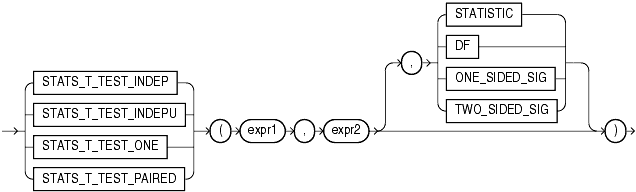
The t-test measures the significance of a difference of means. You can use it to compare the means of two groups or the means of one group with a constant. The STATS_T_TEST_* functions take three arguments: two expressions and a return value of type VARCHAR2. The functions return one number, determined by the value of the third argument. If you omit the third argument, the default is TWO_SIDED_SIG. The meaning of the return values is shown in Table 7-9.
Table 7-9 STATS_T_TEST_* Return Values
| Return Value | Meaning |
|---|---|
STATISTIC |
The observed value of t |
DF |
Degree of freedom |
ONE_SIDED_SIG |
One-tailed significance of t |
TWO_SIDED_SIG |
Two-tailed significance of t |
The significance of the observed value of t is the probability that the value of t would have been obtained by chance—a number between 0 and 1. The smaller the value, the more significant the difference between the means.
The degree of freedom depends on the type of t-test that resulted in the observed value of t. For example, for a one-sample t-test (STATS_T_TEST_ONE), the degree of freedom is the number of observations in the sample minus 1.
In the STATS_T_TEST_ONE function, expr1 is the sample and expr2 is the constant mean against which the sample mean is compared. This function obtains the value of t by dividing the difference between the sample mean and the known mean by the standard error of the mean (rather than the standard error of the difference of the means, as for STATS_T_TEST_PAIRED).
The following example determines the significance of the difference between the average list price and the constant value 60:
SELECT AVG(prod_list_price) group_mean,
       STATS_T_TEST_ONE(prod_list_price, 60, 'STATISTIC') t_observed,
       STATS_T_TEST_ONE(prod_list_price, 60) two_sided_p_value
  FROM sh.products;

GROUP_MEAN T_OBSERVED TWO_SIDED_P_VALUE
---------- ---------- -----------------
139.545556 2.32107746        .023158537
In the STATS_T_TEST_PAIRED function, expr1 and expr2 are the two samples whose means are being compared. This function obtains the value of t by dividing the difference between the sample means by the standard error of the difference of the means (rather than the standard error of the mean, as for STATS_T_TEST_ONE).
In the STATS_T_TEST_INDEP and STATS_T_TEST_INDEPU functions, expr1 is the grouping column and expr2 is the sample of values. The pooled variances version (STATS_T_TEST_INDEP) tests whether the means are the same or different for two distributions that have similar variances. The unpooled variances version (STATS_T_TEST_INDEPU) tests whether the means are the same or different even if the two distributions are known to have significantly different variances.
Before using these functions, it is advisable to determine whether the variances of the samples are significantly different. If they are, then the data may come from distributions with different shapes, and the difference of the means may not be very useful. You can perform an f-test to determine the difference of the variances. If they are not significantly different, use STATS_T_TEST_INDEP. If they are significantly different, use STATS_T_TEST_INDEPU. Please refer to STATS_F_TEST for information on performing an f-test.
The following example determines the significance of the difference between the average sales to men and women where the distributions are assumed to have similar (pooled) variances:
SELECT SUBSTR(cust_income_level, 1, 22) income_level,
       AVG(DECODE(cust_gender, 'M', amount_sold, null)) sold_to_men,
       AVG(DECODE(cust_gender, 'F', amount_sold, null)) sold_to_women,
       STATS_T_TEST_INDEP(cust_gender, amount_sold, 'STATISTIC') t_observed,
       STATS_T_TEST_INDEP(cust_gender, amount_sold) two_sided_p_value
  FROM sh.customers c, sh.sales s
  WHERE c.cust_id = s.cust_id
  GROUP BY ROLLUP(cust_income_level);

INCOME_LEVEL           SOLD_TO_MEN SOLD_TO_WOMEN T_OBSERVED TWO_SIDED_P_VALUE
---------------------- ----------- ------------- ---------- -----------------
A: Below 30,000          105.28349    99.4281447 -1.9880629        .046811482
B: 30,000 - 49,999       102.59651    109.829642 3.04330875        .002341053
C: 50,000 - 69,999      105.627588    110.127931 2.36148671        .018204221
D: 70,000 - 89,999      106.630299     110.47287 2.28496443        .022316997
E: 90,000 - 109,999     103.396741    101.610416 -1.2544577        .209677823
F: 110,000 - 129,999     106.76476    105.981312 -.60444998        .545545304
G: 130,000 - 149,999    108.877532     107.31377 -.85298245        .393671218
H: 150,000 - 169,999    110.987258    107.152191 -1.9062363        .056622983
I: 170,000 - 189,999    102.808238     107.43556 2.18477851        .028908566
J: 190,000 - 249,999    108.040564    115.343356 2.58313425        .009794516
K: 250,000 - 299,999    112.377993    108.196097 -1.4107871        .158316973
L: 300,000 and above    120.970235    112.216342 -2.0642868        .039003862
                        107.121845     113.80441 .686144393        .492670059
                        106.663769    107.276386 1.08013499        .280082357

14 rows selected.
The following example determines the significance of the difference between the average sales to men and women where the distributions are known to have significantly different (unpooled) variances:
SELECT SUBSTR(cust_income_level, 1, 22) income_level,
       AVG(DECODE(cust_gender, 'M', amount_sold, null)) sold_to_men,
       AVG(DECODE(cust_gender, 'F', amount_sold, null)) sold_to_women,
       STATS_T_TEST_INDEPU(cust_gender, amount_sold, 'STATISTIC') t_observed,
       STATS_T_TEST_INDEPU(cust_gender, amount_sold) two_sided_p_value
  FROM sh.customers c, sh.sales s
  WHERE c.cust_id = s.cust_id
  GROUP BY ROLLUP(cust_income_level);

INCOME_LEVEL           SOLD_TO_MEN SOLD_TO_WOMEN T_OBSERVED TWO_SIDED_P_VALUE
---------------------- ----------- ------------- ---------- -----------------
A: Below 30,000          105.28349    99.4281447 -2.0542592        .039964704
B: 30,000 - 49,999       102.59651    109.829642 2.96922332        .002987742
C: 50,000 - 69,999      105.627588    110.127931  2.3496854        .018792277
D: 70,000 - 89,999      106.630299     110.47287 2.26839281        .023307831
E: 90,000 - 109,999     103.396741    101.610416 -1.2603509        .207545662
F: 110,000 - 129,999     106.76476    105.981312 -.60580011        .544648553
G: 130,000 - 149,999    108.877532     107.31377 -.85219781        .394107755
H: 150,000 - 169,999    110.987258    107.152191 -1.9451486        .051762624
I: 170,000 - 189,999    102.808238     107.43556 2.14966921        .031587875
J: 190,000 - 249,999    108.040564    115.343356 2.54749867        .010854966
K: 250,000 - 299,999    112.377993    108.196097 -1.4115514        .158091676
L: 300,000 and above    120.970235    112.216342 -2.0726194        .038225611
                        107.121845     113.80441 .689462437        .490595765
                        106.663769    107.276386 1.07853782        .280794207

14 rows selected.
|
 Copyright © 1996, 2003 Oracle Corporation All Rights Reserved. |
|

